Experiment 2.3: Explicit normalization
In Ex 2.2, we applied interventions to the trained, structured color autoencoder — successfully impeding the models capability to operate on the concept of red. While it worked to some extent, the latent space looked lumpy, and — since the interventions assume the activations have unit length — we expect the performance will benefit from explicit normalization.
Our autoencoders up until now have had a sigmoid function applied to the output of the decoder, to force the values to be in the range $(0,1)$. But this is incorrect, because RGB components should be in the range $[0,1]$ (inclusive).
Hypothesis 1: We're asking too much of the unit norm regularizer
If we weakly regularize latent activations to have unit norm, and then explicity normalize them, then the reconstruction capabilities of the model will be better, and the interventions will be more accurate.
Hypothesis 2: Sigmoid harms performance
If we remove the sigmoid layer, then the reconstruction capabilities of the model will be better.
from __future__ import annotations

nbid = '2.3'  # ID for tagging assets
nbname = 'Explicit norm'
experiment_name = f'Ex {nbid}: {nbname}'
project = 'ex-preppy'
# Basic setup: Logging, Experiment (Modal)
import logging

import modal

from infra.requirements import freeze, project_packages
from mini.experiment import Experiment
from utils.logging import SimpleLoggingConfig

logging_config = (
    SimpleLoggingConfig()
    .info('notebook', 'utils', 'mini', 'ex_color')
    .error('matplotlib.axes')  # Silence warnings about set_aspect
)
logging_config.apply()

# This is the logger for this notebook
log = logging.getLogger(f'notebook.{nbid}')

run = Experiment(experiment_name, project=project)
run.image = modal.Image.debian_slim().pip_install(*freeze(all=True)).add_local_python_source(*project_packages())
run.before_each(logging_config.apply)
None  # prevent auto-display of this cell
Regularizers
Like Ex 2.2:
- Anchor: pins
redto $(1,0,0,0)$ - Separate: angular repulsion to reduce global clumping (applied within each batch)
- Planarity: pulls vibrant hues to the $[0, 1]$ plane
- Unitarity: pulls all embeddings to the surface of the unit hypersphere, i.e. it makes the embedding vectors have unit length.
But unlike previous experiments:
- Unitarity: we now only have one unitarity term, which is applied very weakly to the outputs of the encoder. Previously there were two terms and they were stronger (because the model didn't explicitly normalize the activations).
Why have a unitarity regularizer at all, if the activations are explicitly normalized? Because this gives the upstream layers a hint about what the downstream layers expect — otherwise that signal would be destroyed by the normalization.
import torch

from mini.temporal.dopesheet import Dopesheet
from ex_color.loss import Anchor, Separate, Planarity, Unitarity, RegularizerConfig

from ex_color.training import TrainingModule

RED = (1, 0, 0, 0)

ALL_REGULARIZERS = [
    RegularizerConfig(
        name='reg-unit',
        compute_loss_term=Unitarity(),
        label_affinities=None,
        layer_affinities=['encoder'],
    ),
    RegularizerConfig(
        name='reg-anchor',
        compute_loss_term=Anchor(torch.tensor(RED, dtype=torch.float32)),
        label_affinities={'red': 1.0},
        layer_affinities=['encoder'],
    ),
    RegularizerConfig(
        name='reg-separate',
        compute_loss_term=Separate(power=100.0, shift=True),
        label_affinities=None,
        layer_affinities=['encoder'],
    ),
    RegularizerConfig(
        name='reg-planar',
        compute_loss_term=Planarity(),
        label_affinities={'vibrant': 1.0},
        layer_affinities=['encoder'],
    ),
]


import logging
from typing import override

import torch.nn as nn
from torch import Tensor

log = logging.getLogger(__name__)


class CNColorMLP(nn.Module):
    """A clamped-and-normalized RGB-to-RGB bottlenecked autoencoder"""

    def __init__(self, k_bottleneck: int, sigmoid_out: bool):
        super().__init__()
        # RGB input (3D) → hidden layer → bottleneck → hidden layer → RGB output
        self.encoder = nn.Sequential(
            nn.Linear(3, 16),
            nn.GELU(),
            nn.Linear(16, k_bottleneck),
        )

        self.bottleneck = L2Norm()

        self.decoder = nn.Sequential(
            nn.Linear(k_bottleneck, 16),
            nn.GELU(),
            nn.Linear(16, 3),
            nn.Sigmoid() if sigmoid_out else nn.Identity(),
        )

    @override  # Overridden to narrow types
    def __call__(self, x: Tensor) -> Tensor:
        return super().__call__(x)

    @override
    def forward(self, x: Tensor) -> Tensor:
        # Get the bottleneck representation (captured by a hook for regularization)
        x = self.encoder(x)

        # Normalize
        x = self.bottleneck(x)

        # Decode back to RGB
        x = self.decoder(x)
        return x if self.training else torch.clamp(x, 0, 1)


class L2Norm(nn.Module):
    def forward(self, x: Tensor):
        return nn.functional.normalize(x, dim=-1)


def make_model(sigmoid_out: bool):
    return CNColorMLP(4, sigmoid_out)
from functools import partial
from torch import Tensor
from torch.utils.data import DataLoader, TensorDataset, WeightedRandomSampler
import numpy as np

from ex_color.data.color_cube import ColorCube
from ex_color.data.cube_sampler import vibrancy
from ex_color.data.cyclic import arange_cyclic
from ex_color.labelling import collate_with_generated_labels


def prep_data() -> tuple[DataLoader, Tensor]:
    """
    Prepare data for training.

    Returns: (train, val)
    """
    hsv_cube = ColorCube.from_hsv(
        h=arange_cyclic(step_size=10 / 360),
        s=np.linspace(0, 1, 10),
        v=np.linspace(0, 1, 10),
    )
    hsv_tensor = torch.tensor(hsv_cube.rgb_grid.reshape(-1, 3), dtype=torch.float32)
    vibrancy_tensor = torch.tensor(vibrancy(hsv_cube).flatten(), dtype=torch.float32)
    hsv_dataset = TensorDataset(hsv_tensor, vibrancy_tensor)

    labeller = partial(
        collate_with_generated_labels,
        soft=False,  # Use binary labels (stochastic) to simulate the labelling of internet text
        red=0.5,
        vibrant=0.5,
    )
    # Desaturated and dark colors are over-represented in the cube, so we use a weighted sampler to balance them out
    hsv_loader = DataLoader(
        hsv_dataset,
        batch_size=64,
        num_workers=2,
        sampler=WeightedRandomSampler(
            weights=hsv_cube.bias.flatten().tolist(),
            num_samples=len(hsv_dataset),
            replacement=True,
        ),
        collate_fn=labeller,
    )

    rgb_cube = ColorCube.from_rgb(
        r=np.linspace(0, 1, 8),
        g=np.linspace(0, 1, 8),
        b=np.linspace(0, 1, 8),
    )
    rgb_tensor = torch.tensor(rgb_cube.rgb_grid.reshape(-1, 3), dtype=torch.float32)
    return hsv_loader, rgb_tensor
import wandb
from ex_color.inference import InferenceModule
from ex_color.intervention.intervention import InterventionConfig


# @run.thither(env={'WANDB_API_KEY': wandb.Api().api_key})
async def train(
    dopesheet: Dopesheet,
    regularizers: list[RegularizerConfig],
    sigmoid_out: bool,
) -> CNColorMLP:
    """Train the model with the given dopesheet and variant."""
    import lightning as L
    from lightning.pytorch.loggers import WandbLogger

    from ex_color.seed import set_deterministic_mode

    from utils.progress.lightning import LightningProgress

    log.info(f'Training with: {[r.name for r in regularizers]}')

    seed = 0
    set_deterministic_mode(seed)

    hsv_loader, _ = prep_data()

    model = make_model(sigmoid_out)
    total_params = sum(p.numel() for p in model.parameters() if p.requires_grad)
    log.debug(f'Model initialized with {total_params:,} trainable parameters.')

    training_module = TrainingModule(model, dopesheet, torch.nn.MSELoss(), regularizers)

    logger = WandbLogger(experiment_name + (', sigmoid' if sigmoid_out else ', linear'), project=project)

    trainer = L.Trainer(
        max_steps=len(dopesheet),
        callbacks=[
            LightningProgress(),
        ],
        enable_checkpointing=False,
        enable_model_summary=False,
        # enable_progress_bar=True,
        logger=logger,
    )

    print(f'max_steps: {len(dopesheet)}, hsv_loader length: {len(hsv_loader)}')

    # Train the model
    try:
        trainer.fit(training_module, hsv_loader)
    finally:
        wandb.finish()
    # This is only a small model, so it's OK to return it rather than storing and loading a checkpoint remotely
    return model
async with run():
    model_sigmoid = await train(Dopesheet.from_csv(f'./ex-{nbid}-dopesheet.csv'), ALL_REGULARIZERS, sigmoid_out=True)
INFO: Seed set to 0
I 6.3 li.fa.ut.se:Seed set to 0
I 6.3 ex.se:   PyTorch set to deterministic mode
INFO: GPU available: False, used: False
I 6.4 li.py.ut.ra:GPU available: False, used: False
INFO: TPU available: False, using: 0 TPU cores
I 6.4 li.py.ut.ra:TPU available: False, using: 0 TPU cores
INFO: HPU available: False, using: 0 HPUs
I 6.4 li.py.ut.ra:HPU available: False, using: 0 HPUs
max_steps: 3001, hsv_loader length: 57
wandb: Currently logged in as: z0r to https://api.wandb.ai. Use `wandb login --relogin` to force relogin
./wandb/run-20250905_065249-qjodfyjo
Starting phase: Train
INFO: `Trainer.fit` stopped: `max_steps=3001` reached.
I 26.9 li.py.ut.ra:`Trainer.fit` stopped: `max_steps=3001` reached.
Run history:
| epoch | ▁▁▁▂▂▂▂▂▂▃▃▃▃▃▄▄▄▄▄▅▅▅▅▅▅▆▆▆▆▆▇▇▇▇▇▇████ |
| train_loss | ▇▄▄▇▅▄▄▄▇▃▄▇█▃▅▄▃▄▂▃▂▄▂▃▄▂▂▁▂▂▁▁▁▁▁▁▁▁▁▁ |
| train_recon | █▃▃▂▂▂▄▂▂▂▅▄▄▅▂▃▃▃▂▃▂▂▂▂▂▁▁▁▁▁▁▁▁▁▁▁▁▁▁▁ |
| train_reg-anchor | ▁▁▁▁▁█▁▁▁▁▅▁▁▁▁▁▁▁▁▁▁▁▁▁▁▁▁▁▁▁▂▂▁▁▂▁▁▂▁▁ |
| train_reg-planar | ▂▄▁▆▆▃▁▁█▁▁▆▁▆▂▂▁▁▂▁▁▂▁▄▃▁▁▁▁▁▁▂▂▁▁▁▁▂▂▂ |
| train_reg-separate | ▃▃▃▃▂▄▃▂▁▂▂█▃▂▂▂▁▂▂▂▁▂▃▂▁▂▂▂▁▂▂▂▁▂▁▂▂▃▂▃ |
| train_reg-unit | █▇▆▆▄▁▁▁▁▁▁▁▁▁▁▁▁▁▁▁▁▁▁▁▁▁▁▁▁▁▁▁▁▁▁▁▁▁▁▁ |
| trainer/global_step | ▁▁▁▁▂▂▂▂▂▃▃▃▃▃▃▄▄▄▄▄▅▅▅▅▅▆▆▆▆▆▆▆▆▇▇▇▇███ |
Run summary:
| epoch | 52 |
| train_loss | 0.00019 |
| train_recon | 0.00019 |
| train_reg-anchor | 0 |
| train_reg-planar | 0.03255 |
| train_reg-separate | 0.45008 |
| train_reg-unit | 0.00431 |
| trainer/global_step | 2999 |
View project at: https://wandb.ai/z0r/ex-color-transformer
Synced 5 W&B file(s), 0 media file(s), 0 artifact file(s) and 0 other file(s)
./wandb/run-20250905_065249-qjodfyjo/logs
async with run():
    model = await train(Dopesheet.from_csv(f'./ex-{nbid}-dopesheet.csv'), ALL_REGULARIZERS, sigmoid_out=False)
INFO: Seed set to 0
I 29.2 li.fa.ut.se:Seed set to 0
I 29.2 ex.se:  PyTorch set to deterministic mode
INFO: GPU available: False, used: False
I 29.3 li.py.ut.ra:GPU available: False, used: False
INFO: TPU available: False, using: 0 TPU cores
I 29.3 li.py.ut.ra:TPU available: False, using: 0 TPU cores
INFO: HPU available: False, using: 0 HPUs
I 29.3 li.py.ut.ra:HPU available: False, using: 0 HPUs
max_steps: 3001, hsv_loader length: 57
./wandb/run-20250905_065311-8r5o2ag3
Starting phase: Train
INFO: `Trainer.fit` stopped: `max_steps=3001` reached.
I 48.0 li.py.ut.ra:`Trainer.fit` stopped: `max_steps=3001` reached.
Run history:
| epoch | ▁▁▁▂▂▂▂▂▂▂▃▃▃▃▃▄▄▄▄▄▅▅▅▅▅▆▆▆▆▆▇▇▇▇▇▇▇███ |
| train_loss | █▄▄▆▅▄▄▃▄▃▇▅▃▃▅▃▂▃▄▄▃▃▂▃▂▂▂▂▁▁▁▁▁▁▁▁▁▁▁▁ |
| train_recon | █▂▂▂▁▂▂▁▁▂▂▂▂▂▂▂▁▂▃▁▁▂▁▁▁▁▁▁▁▁▁▁▁▁▁▁▁▁▁▁ |
| train_reg-anchor | ▁▁▁▁█▁▃▁▁▁▃▁▁▁▁▁▁▁▁▁▁▁▁▁▁▁▁▁▁▃▁▁▁▁▃▁▁▃▁▁ |
| train_reg-planar | ▄▃▁█▁▁▃▁▁▂▁▁▄▂▃▄▁▂▁▃▁▁▄▁▃▄▁▂▁▁▁▁▁▃▂▁▃▁▃▃ |
| train_reg-separate | ▃▂▃▂▂▃▅▂▂▂▂▂▂▂█▂▂▂▂▁▁▂▃▁▂▂▂▁▁▂▁▁▁▂▁▁▁▂▂▂ |
| train_reg-unit | ██▇▅▄▂▂▁▁▁▁▁▁▁▁▁▁▁▁▁▁▁▁▁▁▁▁▁▁▁▁▁▁▁▁▁▁▁▁▁ |
| trainer/global_step | ▁▁▁▂▂▂▂▂▂▂▃▃▃▃▃▄▄▄▄▄▅▅▅▅▅▅▆▆▆▆▆▇▇▇▇▇▇███ |
Run summary:
| epoch | 52 |
| train_loss | 2e-05 |
| train_recon | 2e-05 |
| train_reg-anchor | 0 |
| train_reg-planar | 0.05697 |
| train_reg-separate | 0.41534 |
| train_reg-unit | 0.00611 |
| trainer/global_step | 2999 |
View project at: https://wandb.ai/z0r/ex-color-transformer
Synced 5 W&B file(s), 0 media file(s), 0 artifact file(s) and 0 other file(s)
./wandb/run-20250905_065311-8r5o2ag3/logs
# @run.thither
async def infer(
    model: CNColorMLP,
    interventions: list[InterventionConfig],
    test_data: Tensor,
) -> Tensor:
    """Run inference with the given model and interventions."""
    import lightning as L

    inference_module = InferenceModule(model, interventions)
    trainer = L.Trainer(
        enable_checkpointing=False,
        enable_model_summary=False,
        enable_progress_bar=True,
    )
    reconstructed_colors_batches = trainer.predict(
        inference_module,
        DataLoader(
            TensorDataset(test_data.reshape((-1, 3))),
            batch_size=64,
            collate_fn=lambda batch: torch.stack([row[0] for row in batch], 0),
        ),
    )
    assert reconstructed_colors_batches is not None
    # Flatten the list of batches to a single list of tensors
    reconstructed_colors = [item for batch in reconstructed_colors_batches for item in batch]
    # Reshape to match input
    return torch.cat(reconstructed_colors).reshape(test_data.shape)
from IPython.display import clear_output

from utils.nb import displayer_mpl
from ex_color.vis import plot_colors


hsv_cube = ColorCube.from_hsv(
    h=arange_cyclic(step_size=1 / 24),
    s=np.linspace(0, 1, 4),
    v=np.linspace(0, 1, 8),
).permute('svh')
x_hsv = torch.tensor(hsv_cube.rgb_grid, dtype=torch.float32)

hd_hsv_cube = ColorCube.from_hsv(
    h=arange_cyclic(step_size=1 / 240),
    s=np.linspace(0, 1, 48),
    v=np.linspace(0, 1, 48),
)
hd_x_hsv = torch.tensor(hd_hsv_cube.rgb_grid, dtype=torch.float32)

rgb_cube = ColorCube.from_rgb(
    r=np.linspace(0, 1, 20),
    g=np.linspace(0, 1, 20),
    b=np.linspace(0, 1, 20),
)
x_rgb = torch.tensor(rgb_cube.rgb_grid, dtype=torch.float32)

clear_output()

with displayer_mpl(
    f'large-assets/ex-{nbid}-true-colors.png',
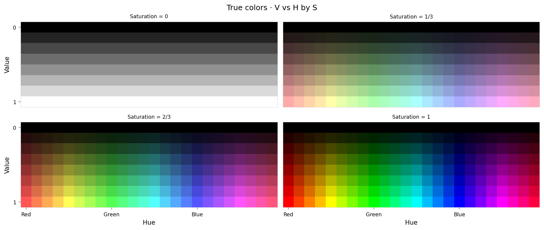
    alt_text="""Plot showing four slices of the HSV cube, titled "{title}". Each slice has constant saturation, but varies in value (brightness) from top to bottom, and in hue from left to right. The first slice shows a grayscale gradient from black to white; the last shows the fully-saturated color spectrum.""",
) as show:
    show(lambda: plot_colors(hsv_cube, title='True colors', colors=x_hsv.numpy()))
from IPython.display import clear_output
from torch.nn import functional as F

from ex_color.vis import plot_colors, plot_cube_series


interventions = []
y_hsv = await infer(model_sigmoid, interventions, x_hsv)
hd_y_hsv = await infer(model_sigmoid, interventions, hd_x_hsv)
clear_output()

with displayer_mpl(
    f'large-assets/ex-{nbid}-pred-colors-no-interventio-sigmoid.png',
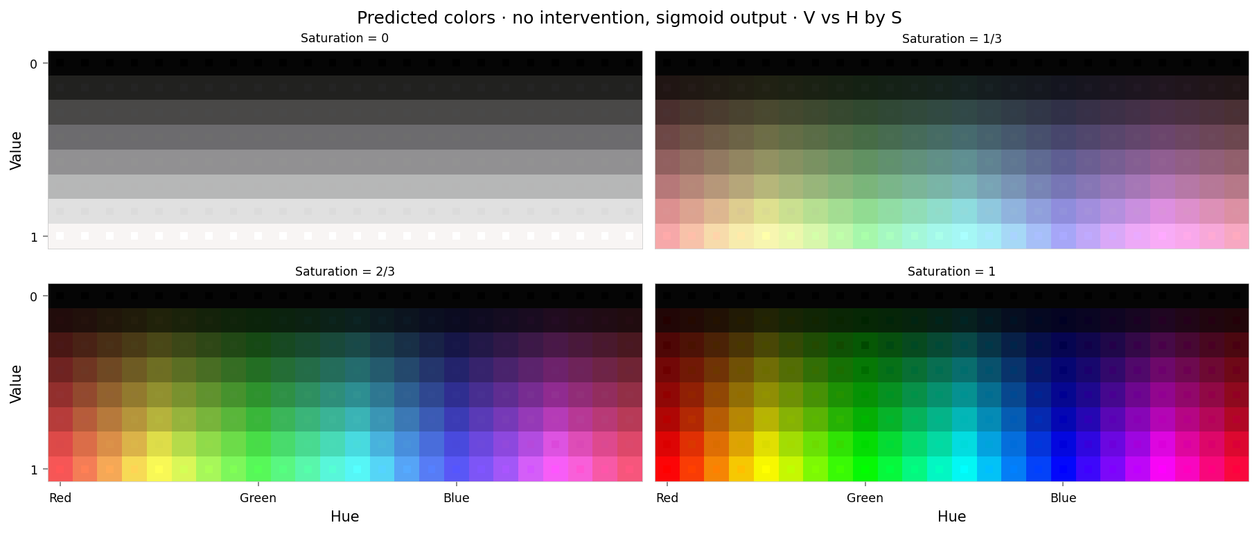
    alt_text="""Plot showing four slices of the HSV cube, titled "{title}". Nominally, each slice has constant saturation, but varies in value (brightness) from top to bottom, and in hue from left to right. Each color value is represented as a square patch of that color. The outer portion of the patches shows the color as reconstructed by the model; the inner portion shows the true (input) color. The reconstructed and true colors agree somewhat, but some differences are visible; for example, "white" is slightly gray, and many of the fully-saturated colors are less saturated than they should be.""",
) as show:
    show(
        lambda: plot_colors(
            hsv_cube,
            title='Predicted colors · no intervention, sigmoid output',
            colors=y_hsv.numpy(),
            colors_compare=x_hsv.numpy(),
        )
    )


per_color_loss = F.mse_loss(hd_y_hsv, hd_x_hsv, reduction='none').mean(dim=-1)
loss_cube = hd_hsv_cube.assign('MSE', per_color_loss.numpy().reshape(hd_hsv_cube.shape))
max_loss = per_color_loss.max().item()
median_loss = per_color_loss.median().item()
with displayer_mpl(
    f'large-assets/ex-{nbid}-loss-colors-no-intervention-sigmoid.png',
    alt_text=f"""Line chart showing loss per color, titled "{{title}}". Y-axis: mean square error, ranging from zero to {max_loss:.2g}. X-axis: hue. There is a lot of variation; the lines of color are quite messy.""",
) as show:
    show(
        lambda: plot_cube_series(
            loss_cube.permute('hsv')[:, -1:, :: (loss_cube.shape[2] // -5)],
            loss_cube.permute('svh')[:, -1:, :: -(loss_cube.shape[0] // -3)],
            loss_cube.permute('vsh')[:, -1:, :: -(loss_cube.shape[0] // -3)],
            title='Reconstruction error · no intervention, sigmoid output',
            var='MSE',
            figsize=(12, 3),
        )
    )
print(f'Max MSE: {max_loss:.2g}')
print(f'Median MSE: {median_loss:.2g}')

Max MSE: 0.0016
Median MSE: 6.3e-05
OK, that looks similar to the output of Ex 2.2. The reconstruction loss curves look a lot messier, but the range is much smaller — by roughly an order of magnitude.
import torch

from ex_color.inference import InferenceModule


async def infer_with_latent_capture(
    model: CNColorMLP, interventions: list[InterventionConfig], test_data: Tensor, layer_name: str = 'bottleneck'
) -> tuple[Tensor, Tensor]:
    module = InferenceModule(model, interventions, capture_layers=[layer_name])
    import lightning as L

    trainer = L.Trainer(enable_checkpointing=False, enable_model_summary=False, enable_progress_bar=False)
    batches = trainer.predict(
        module,
        DataLoader(
            TensorDataset(test_data.reshape((-1, 3))),
            batch_size=64,
            collate_fn=lambda batch: torch.stack([row[0] for row in batch], 0),
        ),
    )
    assert batches is not None
    preds = [item for batch in batches for item in batch]
    y = torch.cat(preds).reshape(test_data.shape)
    # Read captured activations as a flat [N, D] tensor
    latents = module.read_captured(layer_name)
    return y, latents
from IPython.display import clear_output

from ex_color.vis import plot_latent_grid_3d


y_rgb, h_rgb = await infer_with_latent_capture(model_sigmoid, [], x_rgb, 'bottleneck')
clear_output()

with displayer_mpl(
    f'large-assets/ex-{nbid}-latents-no-intervention-sigmoid.png',
    alt_text="""Three spherical plots, titled "{title}". Each plot shows a vibrant collection of colored circles or balls scattered over the surface of a black sphere. The first plot has the appearance of a color wheel, with the full set of vibrant colors around the rim (like a rainbow), varying to black in the center. It's fairly regular but has a couple of bulges. The other plots show different views of the same sphere, with hue varying across the equator and tone varying from top to bottom, and red in the center. Each ball shows the reconstructed color, with a dot in the center showing the true (input) color. In this plot the true and reconstructor colors agree very well, but slight differences can be seen if you look closely.""",
) as show:
    show(
        lambda theme: plot_latent_grid_3d(
            h_rgb,
            y_rgb,
            x_rgb,
            title='Latents · no intervention, sigmoid',
            dims=[(1, 0, 2), (1, 2, 0), (1, 3, 0)],
            dot_radius=10,
            theme=theme,
        )
    )
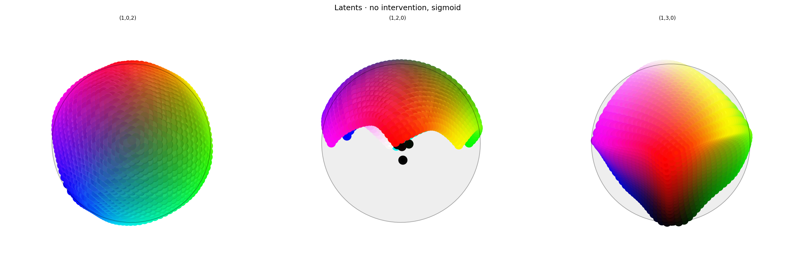
The latent space looks considerably better than Ex 2.2, and only required one tenth the number of training steps. So we're getting an order of magnitude better performance, with an order of magnitude less compute. Not bad.
Can we push it further?
from IPython.display import clear_output
from torch.nn import functional as F

from ex_color.vis import plot_colors, plot_cube_series


interventions = []
y_hsv = await infer(model, interventions, x_hsv)
hd_y_hsv = await infer(model, interventions, hd_x_hsv)
clear_output()

with displayer_mpl(
    f'large-assets/ex-{nbid}-pred-colors-no-intervention.png',
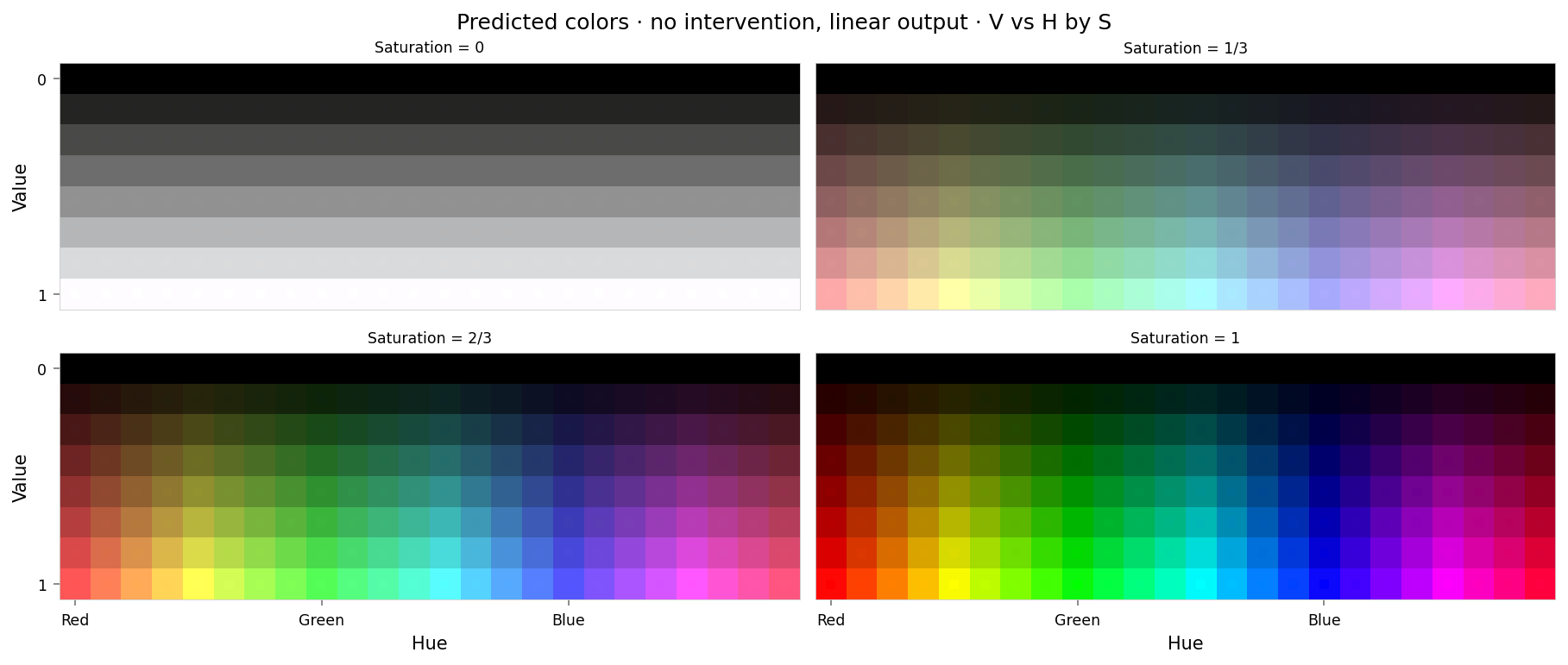
    alt_text="""Plot showing four slices of the HSV cube, titled "{title}". Nominally, each slice has constant saturation, but varies in value (brightness) from top to bottom, and in hue from left to right. Each color value is represented as a square patch of that color. The outer portion of the patches shows the color as reconstructed by the model; the inner portion shows the true (input) color. The reconstructed and true colors agree very well; it's hard to see any differences.""",
) as show:
    show(
        lambda: plot_colors(
            hsv_cube,
            title='Predicted colors · no intervention, linear output',
            colors=y_hsv.numpy(),
            colors_compare=x_hsv.numpy(),
        )
    )


per_color_loss = F.mse_loss(hd_y_hsv, hd_x_hsv, reduction='none').mean(dim=-1)
loss_cube = hd_hsv_cube.assign('MSE', per_color_loss.numpy().reshape(hd_hsv_cube.shape))
max_loss = per_color_loss.max().item()
median_loss = per_color_loss.median().item()
with displayer_mpl(
    f'large-assets/ex-{nbid}-loss-colors-no-intervention.png',
    alt_text=f"""Line chart showing loss per color, titled "{{title}}". Y-axis: mean square error, ranging from zero to {max_loss:.2g}. X-axis: hue. The range of loss values is small and the series are quite neat, but there are two notable peaks at blue and green, and smaller peaks at red and yellow.""",
) as show:
    show(
        lambda: plot_cube_series(
            loss_cube.permute('hsv')[:, -1:, :: (loss_cube.shape[2] // -5)],
            loss_cube.permute('svh')[:, -1:, :: -(loss_cube.shape[0] // -3)],
            loss_cube.permute('vsh')[:, -1:, :: -(loss_cube.shape[0] // -3)],
            title='Reconstruction error · no intervention, linear output',
            var='MSE',
            figsize=(12, 3),
        )
    )
print(f'Max MSE: {max_loss:.2g}')
print(f'Median MSE: {median_loss:.2g}')

Max MSE: 0.0017
Median MSE: 1.6e-05
That's very good: Visually, the reconstructed colors agree extremely well with the true colors. White no longer looks "off-white", and it's hard to see the differences in the fully-saturated colors. The maximum reconstruction loss is about the same as the model that did use sigmoid, but the median loss is smaller by a factor of six — and the curves are less "messy".
from IPython.display import clear_output

from ex_color.vis import plot_latent_grid_3d


y_rgb, h_rgb = await infer_with_latent_capture(model, [], x_rgb, 'bottleneck')
clear_output()

with displayer_mpl(
    f'large-assets/ex-{nbid}-latents-no-intervention.png',
    alt_text="""Three spherical plots, titled "{title}". Each plot shows a vibrant collection of colored circles or balls scattered over the surface of a black sphere. The first plot has the appearance of a color wheel, with the full set of vibrant colors around the rim (like a rainbow), varying to black in the center. It is very regular in shape. The other plots show different views of the same sphere, with hue varying across the equator and tone varying from top to bottom, and red in the center. Each ball shows the reconstructed color, with a dot in the center showing the true (input) color. In this plot the true and reconstructor colors agree very well.""",
) as show:
    show(
        lambda theme: plot_latent_grid_3d(
            h_rgb,
            y_rgb,
            x_rgb,
            title='Latents · no intervention',
            dims=[(1, 0, 2), (1, 2, 0), (1, 3, 0)],
            dot_radius=10,
            theme=theme,
        )
    )
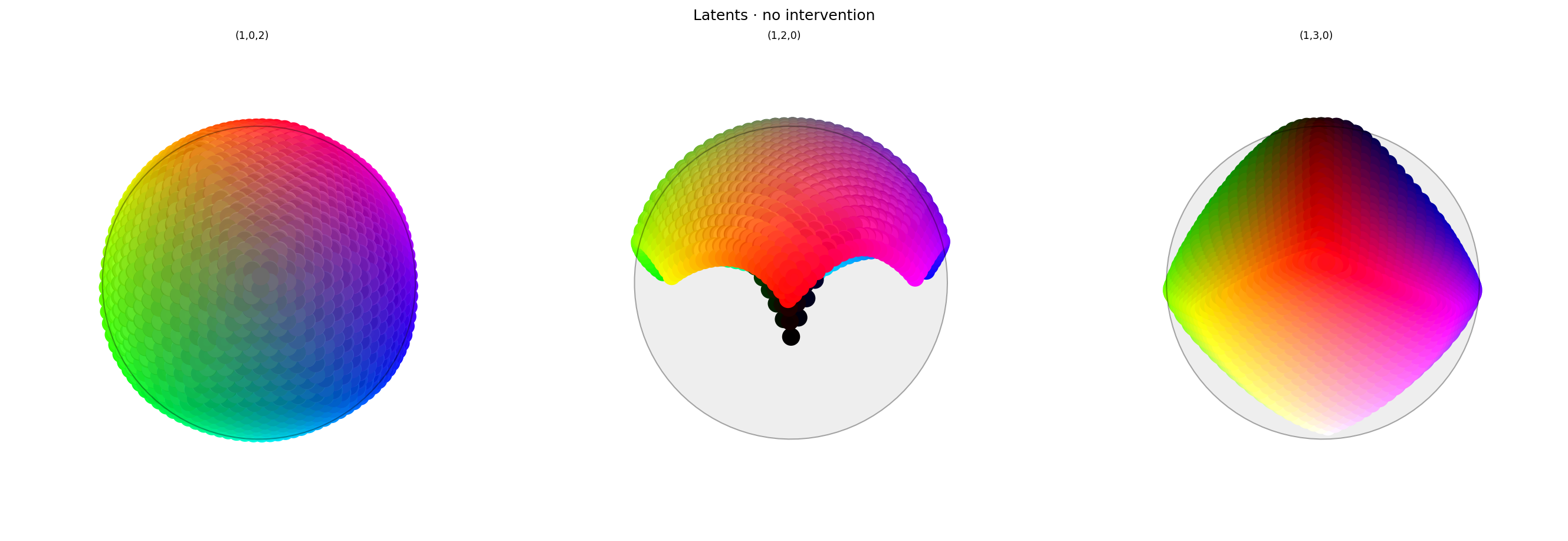
Latent space looks extremely good: very regular and round.
From here on, we'll use the linear model (i.e. without sigmoid applied to the outputs). Let's re-run the suppression and repulsion tests from Ex 2.2 with this model.
Suppression
Now that we have our model, let's try suppressing red. We'll use the Suppression function developed in Ex 2.1.
from math import cos, pi

import torch

from ex_color.intervention import BoundedFalloff, InterventionConfig, Suppression
from ex_color.vis import plot_colors, plot_cube_series


suppression = Suppression(
    torch.tensor(RED, dtype=torch.float32),  # Constant!
    BoundedFalloff(
        0,  # within 60°
        1,  # completely squash fully-aligned vectors
        2,  # soft rim, sharp hub
    ),
)

interventions = [InterventionConfig(suppression, ['bottleneck'])]
y_hsv = await infer(model, interventions, x_hsv)
hd_y_hsv = await infer(model, interventions, hd_x_hsv)
clear_output()

with displayer_mpl(
    f'large-assets/ex-{nbid}-pred-colors-suppression.png',
    alt_text="""Plot showing four slices of the HSV cube, titled "{{title}}". Nominally, each slice has constant saturation, but varies in value (brightness) from top to bottom, and in hue from left to right. Each color value is represented as a square patch of that color. The outer portion of the patches shows the color as reconstructed by the model; the inner portion shows the true (input) color. The reconstructed and true colors agree fairly well, but "red" and nearby colors are clearly different: red itself appears as middle-gray, and the surrounding colors up to orange and pink look washed out. "Red-orange" actually appears to be green, moreso even than yellow (which is geometrically closer to green).""",
) as show:
    show(
        lambda: plot_colors(
            hsv_cube,
            title='Predicted colors with suppression',
            colors=y_hsv.numpy(),
            colors_compare=x_hsv.numpy(),
        )
    )


per_color_loss = F.mse_loss(hd_y_hsv, hd_x_hsv, reduction='none').mean(dim=-1)
loss_cube = hd_hsv_cube.assign('MSE', per_color_loss.numpy().reshape(hd_hsv_cube.shape))
max_loss = per_color_loss.max().item()
median_loss = per_color_loss.median().item()
with displayer_mpl(
    f'large-assets/ex-{nbid}-loss-colors-suppression.png',
    alt_text=f"""Line chart showing loss per color, titled "{{title}}". Y-axis: mean square error, ranging from zero to {max_loss:.2g}. X-axis: hue. There is a significant peak at red at either end of the X-axis, gradually sloping down to lower loss values near yellow and pink. Two very small peaks are at green and blue (apparently around 1% of the height of the peaks at red).""",
) as show:
    show(
        lambda: plot_cube_series(
            loss_cube.permute('hsv')[:, -1:, :: (loss_cube.shape[2] // -5)],
            loss_cube.permute('svh')[:, -1:, :: -(loss_cube.shape[0] // -6)],
            loss_cube.permute('vsh')[:, -1:, :: -(loss_cube.shape[0] // -6)],
            title='Reconstruction error · suppression',
            var='MSE',
            figsize=(12, 3),
        )
    )
print(f'Max MSE: {max_loss:.2g}')
print(f'Median MSE: {median_loss:.2g}')
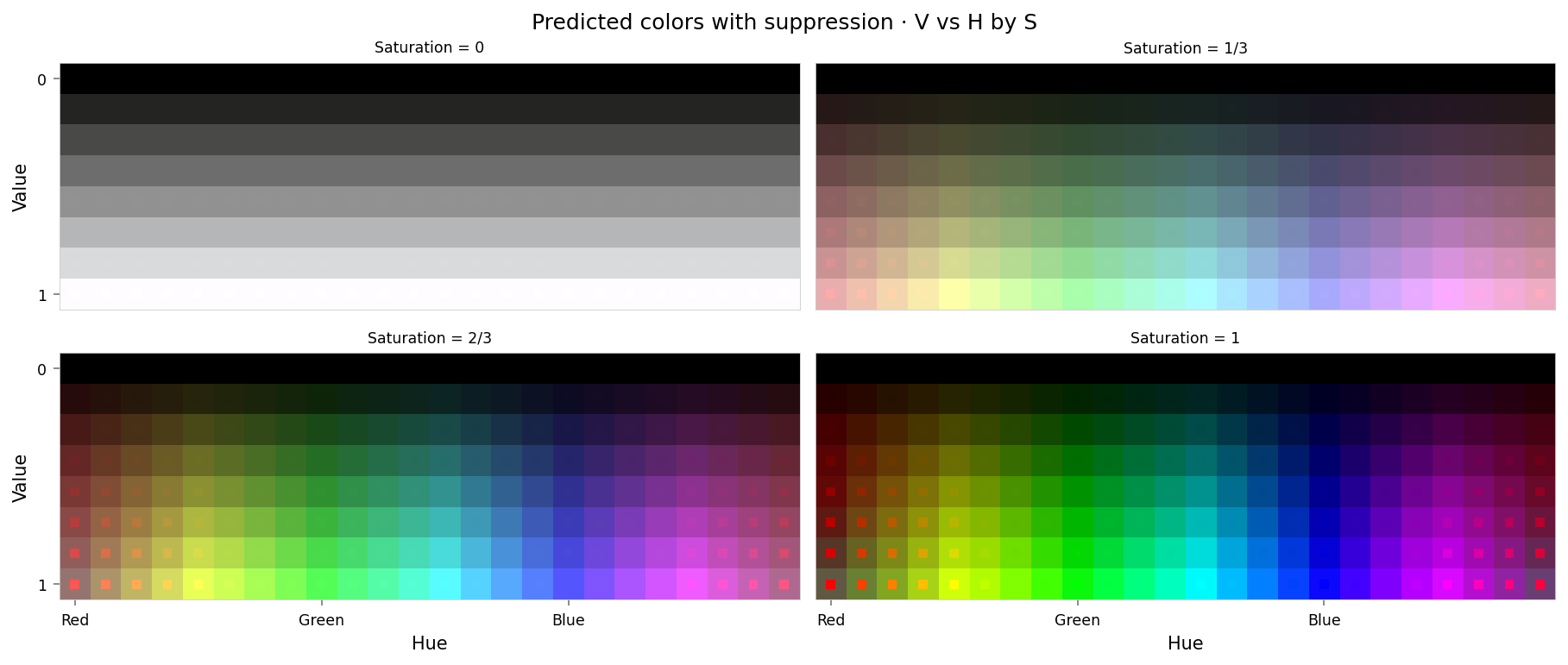

Max MSE: 0.19
Median MSE: 1.9e-05
This looks good — much like the suppression results from Ex 2.2, but much smoother — which should mean that the intervention would have more predictable effects and be more targeted.
from IPython.display import clear_output

from ex_color.vis import plot_latent_grid_3d, ConicalAnnotation

y_rgb, h_rgb = await infer_with_latent_capture(model, interventions, x_rgb, 'bottleneck')
clear_output()

with displayer_mpl(
    f'large-assets/ex-{nbid}-latents-suppression.png',
    alt_text="""Three spherical plots, titled "{title}". Each plot shows a vibrant collection of colored circles or balls scattered over the surface of a black sphere. The first plot has the appearance of a partial color wheel, with  vibrant colors around the rim (like a rainbow), with with a conspicuously absent space at the top where "red" should be. The other plots show different views of the same sphere, with hue varying across the equator and tone varying from top to bottom, and warm colors in the center. Each ball shows the reconstructed color, with a dot in the center showing the true (input) color. The true and reconstructor colors agree fairly well, even for the warmer colors. "Red" itself is in fact not visible, being buried somewhere inside the sphere.""",
) as show:
    show(
        lambda theme: plot_latent_grid_3d(
            h_rgb,
            y_rgb,
            x_rgb,
            title='Latents · suppression',
            dims=[(1, 0, 2), (1, 2, 0), (1, 3, 0)],
            dot_radius=10,
            theme=theme,
            annotations=[
                ConicalAnnotation(
                    RED,
                    2 * (np.pi / 2 - suppression.falloff.a),  # type: ignore
                    color=theme.val('black', dark='#fffa'),
                    linewidth=theme.val(0.5, dark=1),
                    dashes=theme.val((8, 8), dark=(4, 4)),
                    gapcolor=theme.val('#fff4', dark='#0004'),
                ),
            ],
        )
    )
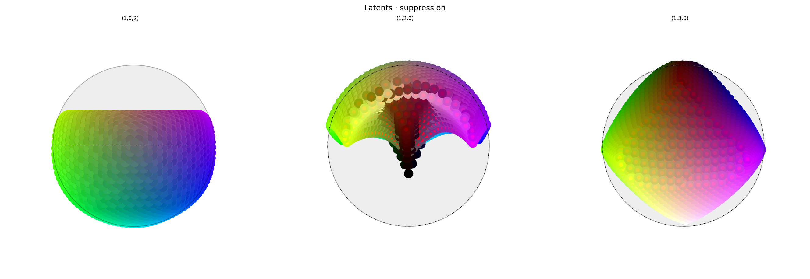
This is really good. Just like in Ex 2.2, the top of the first plot has been pushed in — but it's very regular. The others show the deformation too, with warmer colors in the center. We can see colors close to red in the center of the middle plot, showing significant disagreement with the true colors, as expected.
The interior of the sphere is still out of distribution for the decoder; nevertheless the intervention is causing the kind of reconstruction loss we would expect.
from math import cos, pi

import torch

from ex_color.intervention import FastBezierMapper, InterventionConfig, Repulsion
from ex_color.vis import plot_colors, plot_cube_series

repulsion = Repulsion(
    torch.tensor([1, 0, 0, 0], dtype=torch.float32),  # Constant!
    FastBezierMapper(
        0,  # Constrain effect to within 60° cone
        cos(pi / 3),  # Create 30° hole (negative cone) around concept vector
    ),
)


interventions = [InterventionConfig(repulsion, ['bottleneck'])]
y_hsv = await infer(model, interventions, x_hsv)
hd_y_hsv = await infer(model, interventions, hd_x_hsv)
clear_output()

with displayer_mpl(
    f'large-assets/ex-{nbid}-pred-colors-repulsion.png',
    alt_text="""Plot showing four slices of the HSV cube, titled "{title}". Nominally, each slice has constant saturation, but varies in value (brightness) from top to bottom, and in hue from left to right. Each color value is represented as a square patch of that color. The outer portion of the patches shows the color as reconstructed by the model; the inner portion shows the true (input) color. The reconstructed and true colors agree fairly well, but "red" and nearby colors are clearly different, and different again from how the suppression intervention looked: "red" itself appears as pink or hot pink, and the surrounding colors up to orange and pink look shifted. "Red-orange" actually appears to be fully-saturated yellow. Overall the effect is as though the nearby colors have bled into the neighborhood of red.""",
) as show:
    show(
        lambda: plot_colors(
            hsv_cube,
            title='Predicted colors with repulsion',
            colors=y_hsv.numpy(),
            colors_compare=x_hsv.numpy(),
        )
    )


per_color_loss = F.mse_loss(hd_y_hsv, hd_x_hsv, reduction='none').mean(dim=-1)
loss_cube = hd_hsv_cube.assign('MSE', per_color_loss.numpy().reshape(hd_hsv_cube.shape))
max_loss = per_color_loss.max().item()
with displayer_mpl(
    f'large-assets/ex-{nbid}-loss-colors-repulsion.png',
    alt_text=f"""Line chart showing loss per color, titled "{{title}}". Y-axis: mean square error, ranging from zero to {max_loss:.2g}. X-axis: hue. There is a significant peak at red at either end of the X-axis, gradually sloping down to lower loss values near yellow and pink. Two very small peaks are at green and blue (apparently around 1% of the height of the peaks at red).""",
) as show:
    show(
        lambda: plot_cube_series(
            loss_cube.permute('hsv')[:, -1:, :: (loss_cube.shape[2] // -5)],
            loss_cube.permute('svh')[:, -1:, :: -(loss_cube.shape[0] // -6)],
            loss_cube.permute('vsh')[:, -1:, :: -(loss_cube.shape[0] // -6)],
            title='Reconstruction error · repulsion',
            var='MSE',
            figsize=(12, 3),
        )
    )
print(f'Max MSE: {max_loss:.2g}')
print(f'Median MSE: {median_loss:.2g}')
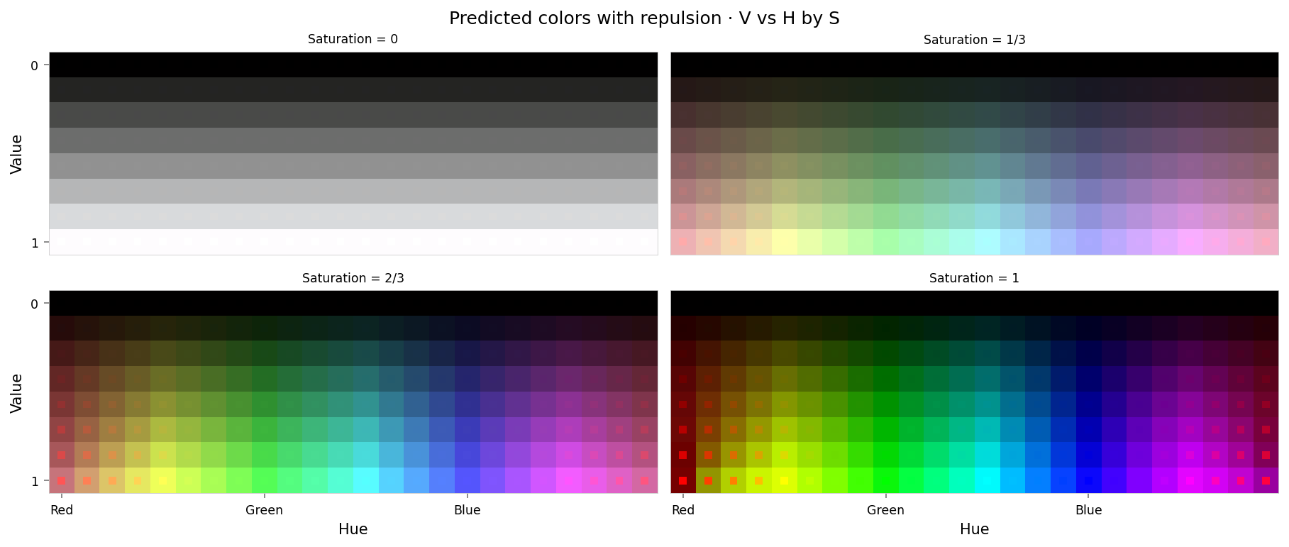

Max MSE: 0.12
Median MSE: 1.9e-05
This looks similar to the suppression result, but the maximum reconstruction loss is lower. That's to be expected, since the repulsion regularizer is configured to push fully-aligned colors 60° away, whereas suppression is configured to squash aligned activations to zero.
The quality of the reconstructed colors is subjectively better to my eyes: red is still red, but darker; whereas with suppression, red shifted to be green. It's hard to say whether that's due to the type of transform or the strength.
from IPython.display import clear_output

from ex_color.vis import plot_latent_grid_3d, ConicalAnnotation

y_rgb, h_rgb = await infer_with_latent_capture(model, interventions, x_rgb, 'bottleneck')
clear_output()

with displayer_mpl(
    f'large-assets/ex-{nbid}-latents-repulsion.png',
    alt_text="""Three spherical plots, titled "{title}". Each plot shows a vibrant collection of colored circles or balls scattered over the surface of a black sphere. The first plot has the appearance of a partial color wheel, with  vibrant colors around the rim (like a rainbow), with with a conspicuously absent space at the top where "red" should be. The other plots show different views of the same sphere, with hue varying across the equator and tone varying from top to bottom. The central region of the second and third plots show something interesting: "Red" and nearby colors have been arranged into a wide ring or disc, rather than being clustered in the center. Each ball shows the reconstructed color, with a dot in the center showing the true (input) color. The true and reconstructor colors agree fairly well, except for colors close to "red", which roughly agree in saturation but differ significantly in tone and hue.""",
) as show:
    show(
        lambda theme: plot_latent_grid_3d(
            h_rgb,
            y_rgb,
            x_rgb,
            title='Latents · repulsion',
            dims=[(1, 0, 2), (1, 2, 0), (1, 3, 0)],
            dot_radius=10,
            theme=theme,
            annotations=[
                ConicalAnnotation(
                    RED,
                    2 * (np.pi / 2 - repulsion.mapper.a),  # type: ignore
                    color=theme.val('black', dark='#fffa'),
                    linewidth=theme.val(0.5, dark=1),
                    dashes=theme.val((8, 8), dark=(4, 4)),
                    gapcolor=theme.val('#fff4', dark='#0004'),
                ),
                ConicalAnnotation(
                    RED,
                    2 * (np.pi / 2 - repulsion.mapper.b),  # type: ignore
                    color=theme.val('black', dark='#fffa'),
                    linewidth=theme.val(0.5, dark=1),
                ),
            ],
        )
    )
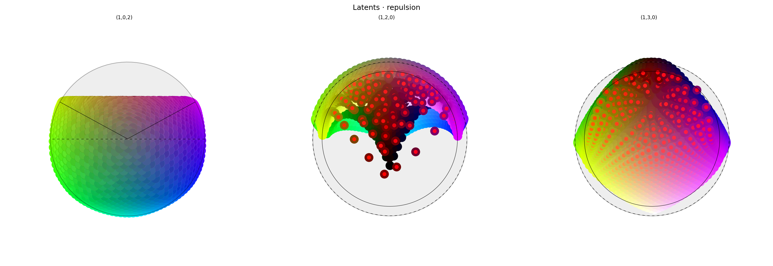
Like in 2.2, red colors have all been pushed away from the intervened-on concept vector, and have formed a ring around it. The effectiveness of this intervention seems similar to the previous model (which lacked explicit normalization). That's surprising: I would have expected repulsion to be more sensitive to deviations from unit norm.
Conclusion
- Explicitly normalizing the bottleneck activations massively improves the reconstruction loss: an order of magnitude better performance with an order of magnitude fewer training steps. The structure of latent space is also much smoother and more regular.
- Removing the sigmoid function from the decoder output helps this model to reproduce colors better, and marginally improves the structure of latent space.
Next steps
See whether performance improves further if some regularizers are run after the explicit normalization.