Experiment 2.2: Specific concept intervention
In the 1.x series of experiments (milestone 1), we validated our ideas for imposing structure on latent space. With only weak supervision, we guided a simple RGB autoencoder to use the color wheel for its latent representations. In this series, we'll try to inhibit and even delete certain concepts from the model.
To start, let's take one of the earlier experiments and see what happens when we suppress activations that align with red.
Hypothesis
We've structured the latent space so red is located at $[1,0,0,0]$. If we suppress or redirect activations close to that vector, model performance on near-red colors should drop, while other colors remain mostly unaffected.
# Basic setup: Logging, Experiment (Modal)
from __future__ import annotations
import logging

import modal

from infra.requirements import freeze, project_packages
from mini.experiment import Experiment
from utils.logging import SimpleLoggingConfig

logging_config = (
    SimpleLoggingConfig()
    .info('notebook', 'utils', 'mini', 'ex_color')
    .error('matplotlib.axes')  # Silence warnings about set_aspect
)
logging_config.apply()

# ID for tagging assets
nbid = '2.2'
# This is the logger for this notebook
log = logging.getLogger(f'notebook.{nbid}')
experiment_name = f'ex-color-{nbid}'

run = Experiment(experiment_name)
run.image = modal.Image.debian_slim().pip_install(*freeze(all=True)).add_local_python_source(*project_packages())
run.before_each(logging_config.apply)
None  # prevent auto-display of this cell
Regularizers
Like Ex 1.7:
- Anchor: pins
redto $(1,0,0,0)$ - Separate: angular repulsion to reduce global clumping (applied within each batch)
- Planarity: pulls vibrant hues to the $[0, 1]$ plane
- Unitarity: pulls all embeddings to the surface of the unit hypersphere, i.e. it makes the embedding vectors have unit length. There are two terms: one that affects all colors equally, and another that just operates on the vibrant colors (because they seemed to need a little more help).
import torch

from mini.temporal.dopesheet import Dopesheet
from ex_color.loss import Anchor, Separate, Planarity, Unitarity, RegularizerConfig
from ex_color.model import ColorMLP
from ex_color.training import TrainingModule

RED = (1, 0, 0, 0)

ALL_REGULARIZERS = [
    RegularizerConfig(
        name='reg-anchor',
        compute_loss_term=Anchor(torch.tensor(RED, dtype=torch.float32)),
        label_affinities={'red': 1.0},
        layer_affinities=['encoder'],
    ),
    RegularizerConfig(
        name='reg-separate',
        compute_loss_term=Separate(power=10.0, shift=False),
        label_affinities=None,
        layer_affinities=['encoder'],
    ),
    RegularizerConfig(
        name='reg-planar',
        compute_loss_term=Planarity(),
        label_affinities={'vibrant': 1.0},
        layer_affinities=['encoder'],
    ),
    RegularizerConfig(
        name='reg-unit-v',
        compute_loss_term=Unitarity(),
        label_affinities={'vibrant': 1.0},
        layer_affinities=['encoder'],
    ),
    RegularizerConfig(
        name='reg-unit',
        compute_loss_term=Unitarity(),
        label_affinities=None,
        layer_affinities=['encoder'],
    ),
]
from functools import partial
from torch import Tensor
from torch.utils.data import DataLoader, TensorDataset, WeightedRandomSampler
import numpy as np

from ex_color.data.color_cube import ColorCube
from ex_color.data.cube_sampler import vibrancy
from ex_color.data.cyclic import arange_cyclic
from ex_color.labelling import collate_with_generated_labels


def prep_data() -> tuple[DataLoader, Tensor]:
    """
    Prepare data for training.

    Returns: (train, val)
    """
    hsv_cube = ColorCube.from_hsv(
        h=arange_cyclic(step_size=10 / 360),
        s=np.linspace(0, 1, 10),
        v=np.linspace(0, 1, 10),
    )
    hsv_tensor = torch.tensor(hsv_cube.rgb_grid.reshape(-1, 3), dtype=torch.float32)
    vibrancy_tensor = torch.tensor(vibrancy(hsv_cube).flatten(), dtype=torch.float32)
    hsv_dataset = TensorDataset(hsv_tensor, vibrancy_tensor)

    labeller = partial(
        collate_with_generated_labels,
        soft=False,  # Use binary labels (stochastic) to simulate the labelling of internet text
        red=0.5,
        vibrant=0.5,
    )
    # Desaturated and dark colors are over-represented in the cube, so we use a weighted sampler to balance them out
    hsv_loader = DataLoader(
        hsv_dataset,
        batch_size=64,
        num_workers=2,
        sampler=WeightedRandomSampler(
            weights=hsv_cube.bias.flatten().tolist(),
            num_samples=len(hsv_dataset),
            replacement=True,
        ),
        collate_fn=labeller,
    )

    rgb_cube = ColorCube.from_rgb(
        r=np.linspace(0, 1, 8),
        g=np.linspace(0, 1, 8),
        b=np.linspace(0, 1, 8),
    )
    rgb_tensor = torch.tensor(rgb_cube.rgb_grid.reshape(-1, 3), dtype=torch.float32)
    return hsv_loader, rgb_tensor
Training
Unlike earlier experiments, we've switched over to use PyTorch Lightning instead of our custom training loop. We also tried porting to Catalyst and Ignite, but we found that Lightning was the closest match to the shape that our training code had evolved into.
Functionally, not much has changed at this point, but now we should be able to take advantage of things like Lightning's distributed processing support.
We have also switched to using Modal for remote compute, and Weights and Biases for experiment tracking. We also tried running our own Aim experiment tracker instance. It worked, but it was slow. We're not sure why; maybe we just hadn't configured the storage or networking properly. If you're curious, check out the aim tag in the Git history.
import wandb
from ex_color.inference import InferenceModule
from ex_color.intervention.intervention import InterventionConfig


# @run.thither(env={'WANDB_API_KEY': wandb.Api().api_key})
async def train(
    dopesheet: Dopesheet,
    regularizers: list[RegularizerConfig],
) -> ColorMLP:
    """Train the model with the given dopesheet and variant."""
    import lightning as L
    from lightning.pytorch.loggers import WandbLogger

    from ex_color.seed import set_deterministic_mode

    from utils.progress.lightning import LightningProgress

    log.info(f'Training with: {[r.name for r in regularizers]}')

    seed = 0
    set_deterministic_mode(seed)

    hsv_loader, _ = prep_data()

    model = ColorMLP(4)
    total_params = sum(p.numel() for p in model.parameters() if p.requires_grad)
    log.debug(f'Model initialized with {total_params:,} trainable parameters.')

    training_module = TrainingModule(model, dopesheet, torch.nn.MSELoss(), regularizers)

    logger = WandbLogger(experiment_name, project='ex-preppy')

    trainer = L.Trainer(
        max_steps=len(dopesheet),
        callbacks=[
            LightningProgress(),
        ],
        enable_checkpointing=False,
        enable_model_summary=False,
        # enable_progress_bar=True,
        logger=logger,
    )

    print(f'max_steps: {len(dopesheet)}, hsv_loader length: {len(hsv_loader)}')

    # Train the model
    try:
        trainer.fit(training_module, hsv_loader)
    finally:
        wandb.finish()
    # This is only a small model, so it's OK to return it rather than storing and loading a checkpoint remotely
    return model


async with run():
    model = await train(Dopesheet.from_csv(f'./ex-{nbid}-dopesheet.csv'), ALL_REGULARIZERS)
I 4.8 no.2.2: Training with: ['reg-anchor', 'reg-separate', 'reg-planar', 'reg-unit-v', 'reg-unit']
INFO: Seed set to 0
I 4.8 li.fa.ut.se:Seed set to 0
I 4.8 ex.se:   PyTorch set to deterministic mode
INFO: GPU available: False, used: False
I 4.8 li.py.ut.ra:GPU available: False, used: False
INFO: TPU available: False, using: 0 TPU cores
I 4.8 li.py.ut.ra:TPU available: False, using: 0 TPU cores
INFO: HPU available: False, using: 0 HPUs
I 4.8 li.py.ut.ra:HPU available: False, using: 0 HPUs
max_steps: 20001, hsv_loader length: 57
wandb: Currently logged in as: z0r to https://api.wandb.ai. Use `wandb login --relogin` to force relogin
./wandb/run-20250905_065602-stbvl7i5
Starting phase: Train
INFO: `Trainer.fit` stopped: `max_steps=20001` reached.
I 124.6 li.py.ut.ra:`Trainer.fit` stopped: `max_steps=20001` reached.
Run history:
| epoch | ▁▁▂▂▂▂▂▂▂▂▃▃▃▃▃▃▄▄▄▄▄▄▄▄▄▅▅▅▅▅▆▆▆▆▆▇▇▇██ |
| train_loss | ▅▇█▇▆▇▇▇█▅▅▃▆▃▃▃▄▂▂▂▁▁▁▁▁▃▁▁▁▁▁▁▁▁▁▁▁▁▁▁ |
| train_recon | ▆▆█▅▅▄▅▂▂▃▂▂▂▃▄▃▂▂▂▂▃▃▂▃▂▁▂▁▁▂▂▁▄▂▁▁▁▂▁▁ |
| train_reg-anchor | ▁▁▁▁▁▁▁▁▁▁▁▁▁▁▁▁▁▁▁▁▁▁▁█▁▁▁▁▁▁▁▁▁▁▂▁▁▁▁▁ |
| train_reg-planar | ▄▂▄▂▄▃█▁█▁▂▁▂▁▁▁▂▁▁▁▁▁▂▂▁▁▁▂▁▁▁▁▁▁▂▁▁▂▁▁ |
| train_reg-separate | ▃▃▃▇▄▁▃▃▂▁▄▂▂▆▄▄▅▃▅▆▇▇▆▅█▆▆▇▇▆▅▇▄▄▄▄▇█▄▅ |
| train_reg-unit | █▆▅▄▄▃▃▃▂▂▁▁▁▁▁▁▁▁▁▁▁▁▁▁▁▁▁▁▁▁▁▁▁▁▁▁▁▁▁▁ |
| train_reg-unit-v | █▅▂▂▁▁▂▁▂▁▁▂▁▃▂▁▂▂▂▂▁▁▁▁▁▁▂▁▁▂▂▁▁▂▁▁▁▁▁▁ |
| trainer/global_step | ▁▁▁▁▁▂▂▂▂▂▂▃▃▃▃▃▃▄▄▄▄▄▅▅▅▅▆▆▆▆▆▆▇▇▇▇████ |
Run summary:
| epoch | 350 |
| train_loss | 0.0043 |
| train_recon | 0.00064 |
| train_reg-anchor | 0 |
| train_reg-planar | 0 |
| train_reg-separate | 3.14612 |
| train_reg-unit | 0.00261 |
| train_reg-unit-v | 0 |
| trainer/global_step | 19999 |
View project at: https://wandb.ai/z0r/ex-color-transformer
Synced 5 W&B file(s), 0 media file(s), 0 artifact file(s) and 0 other file(s)
./wandb/run-20250905_065602-stbvl7i5/logs
# @run.thither
async def infer(
    model: ColorMLP,
    interventions: list[InterventionConfig],
    test_data: Tensor,
) -> Tensor:
    """Run inference with the given model and interventions."""
    import lightning as L

    inference_module = InferenceModule(model, interventions)
    trainer = L.Trainer(
        enable_checkpointing=False,
        enable_model_summary=False,
        enable_progress_bar=True,
    )
    reconstructed_colors_batches = trainer.predict(
        inference_module,
        DataLoader(
            TensorDataset(test_data.reshape((-1, 3))),
            batch_size=64,
            collate_fn=lambda batch: torch.stack([row[0] for row in batch], 0),
        ),
    )
    assert reconstructed_colors_batches is not None
    # Flatten the list of batches to a single list of tensors
    reconstructed_colors = [item for batch in reconstructed_colors_batches for item in batch]
    # Reshape to match input
    return torch.cat(reconstructed_colors).reshape(test_data.shape)
Let's see how well the model reconstructs colors without any interventions.
from IPython.display import clear_output

from utils.nb import displayer_mpl
from ex_color.vis import plot_colors


hsv_cube = ColorCube.from_hsv(
    h=arange_cyclic(step_size=1 / 24),
    s=np.linspace(0, 1, 4),
    v=np.linspace(0, 1, 8),
).permute('svh')
x_hsv = torch.tensor(hsv_cube.rgb_grid, dtype=torch.float32)

hd_hsv_cube = ColorCube.from_hsv(
    h=arange_cyclic(step_size=1 / 240),
    s=np.linspace(0, 1, 48),
    v=np.linspace(0, 1, 48),
)
hd_x_hsv = torch.tensor(hd_hsv_cube.rgb_grid, dtype=torch.float32)

rgb_cube = ColorCube.from_rgb(
    r=np.linspace(0, 1, 20),
    g=np.linspace(0, 1, 20),
    b=np.linspace(0, 1, 20),
)
x_rgb = torch.tensor(rgb_cube.rgb_grid, dtype=torch.float32)

clear_output()

with displayer_mpl(
    f'large-assets/ex-{nbid}-true-colors.png',
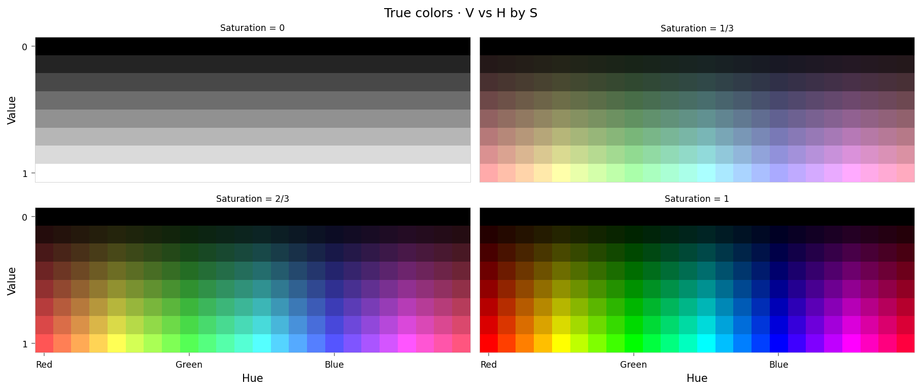
    alt_text="""Plot showing four slices of the HSV cube, titled "True colors - HSV as H,V per S". Each slice has constant saturation, but varies in value (brightness) from top to bottom, and in hue from left to right. The first slice shows a grayscale gradient from black to white; the last shows the fully-saturated color spectrum.""",
) as show:
    show(lambda: plot_colors(hsv_cube, title='True colors', colors=x_hsv.numpy()))
from IPython.display import clear_output
from torch.nn import functional as F

from ex_color.vis import plot_colors, plot_cube_series


interventions = []
y_hsv = await infer(model, interventions, x_hsv)
hd_y_hsv = await infer(model, interventions, hd_x_hsv)
clear_output()

with displayer_mpl(
    f'large-assets/ex-{nbid}-pred-colors-no-intervention.png',
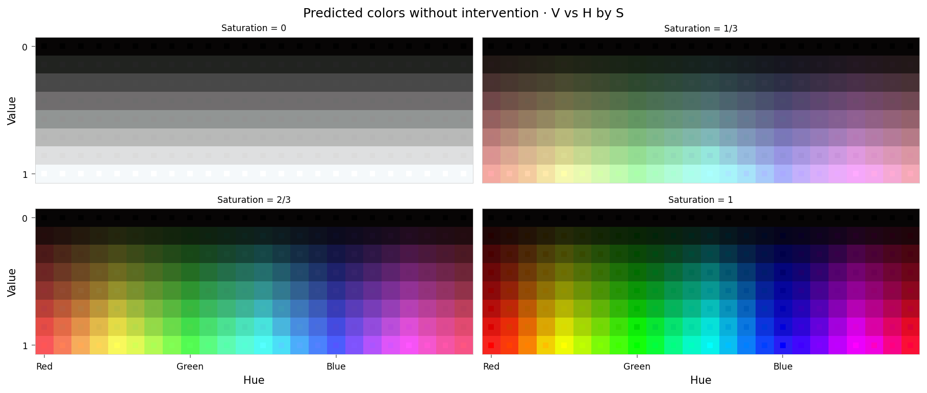
    alt_text="""Plot showing four slices of the HSV cube, titled "Predicted colors without intervention - HSV as H,V per S". Nominally, each slice has constant saturation, but varies in value (brightness) from top to bottom, and in hue from left to right. Each color value is represented as a square patch of that color. The outer portion of the patches shows the color as reconstructed by the model; the inner portion shows the true (input) color. The reconstructed and true colors agree fairly well, but some slight differences are visible; for example, "white" is slightly gray, and many of the fully-saturated colors are less saturated than they should be.""",
) as show:
    show(
        lambda: plot_colors(
            hsv_cube,
            title='Predicted colors without intervention',
            colors=y_hsv.numpy(),
            colors_compare=x_hsv.numpy(),
        )
    )


per_color_loss = F.mse_loss(hd_y_hsv, hd_x_hsv, reduction='none').mean(dim=-1)
loss_cube = hd_hsv_cube.assign('MSE', per_color_loss.numpy().reshape(hd_hsv_cube.shape))
max_loss = per_color_loss.max().item()
with displayer_mpl(
    f'large-assets/ex-{nbid}-loss-colors-no-intervention.png',
    alt_text=f"""Line chart showing loss per color, for colors reconstructed by the model without any intervention. Y-axis: mean square error, ranging from zero to {max_loss:.2g}. X-axis: hue. The range of loss values is small, but there are notable peaks at blue and red. The loss for other colors is low, but varies in a wavy pattern.""",
) as show:
    show(
        lambda: plot_cube_series(
            loss_cube.permute('hsv')[:, -1:, :: (loss_cube.shape[2] // -5)],
            loss_cube.permute('svh')[:, -1:, :: -(loss_cube.shape[0] // -3)],
            loss_cube.permute('vsh')[:, -1:, :: -(loss_cube.shape[0] // -3)],
            title='Reconstruction error · no intervention',
            var='MSE',
            figsize=(12, 3),
        )
    )
print(f'Max MSE: {max_loss:.2g}')

Max MSE: 0.014
That's pretty good: as expected, the reconstructed colors (predictions) look almost the same as the true colors. Visually, the main differences I can see are:
- Fully saturated colors ($s=1$) show some bleeding of green, red, and hot pink into neighboring hues
- Fully desaturated colors ($s=0$) show some hint of being slightly off-gray, i.e. some saturation has crept in.
Sense-check: let's look at the latent space too. We'll use an RGB cube as input for this instead of the HSV cube used above, because it gives a more regular distribution of points — which will be useful to see whether the intervention changes the point density.
import torch

from ex_color.inference import InferenceModule


# Build a tiny helper that runs predict while capturing latents from 'encoder'
async def infer_with_latent_capture(
    model: ColorMLP, interventions: list[InterventionConfig], test_data: Tensor, layer_name: str = 'encoder'
) -> tuple[Tensor, Tensor]:
    module = InferenceModule(model, interventions, capture_layers=[layer_name])
    import lightning as L

    trainer = L.Trainer(enable_checkpointing=False, enable_model_summary=False, enable_progress_bar=False)
    batches = trainer.predict(
        module,
        DataLoader(
            TensorDataset(test_data.reshape((-1, 3))),
            batch_size=64,
            collate_fn=lambda batch: torch.stack([row[0] for row in batch], 0),
        ),
    )
    assert batches is not None
    preds = [item for batch in batches for item in batch]
    y = torch.cat(preds).reshape(test_data.shape)
    # Read captured activations as a flat [N, D] tensor
    latents = module.read_captured(layer_name)
    return y, latents
from IPython.display import clear_output

from ex_color.vis import plot_latent_grid_3d

y_rgb, h_rgb = await infer_with_latent_capture(model, [], x_rgb, 'encoder')
clear_output()

with displayer_mpl(
    f'large-assets/ex-{nbid}-latents-no-intervention.png',
    alt_text="""Three spherical plots, titled "Latents - no intervention". Each plot shows a vibrant collection of colored circles or balls scattered over the surface of a black sphere. The first plot has the appearance of a color wheel, with the full set of vibrant colors around the rim (like a rainbow), varying to black in the center. The other plots show different views of the same sphere, with hue varying across the equator and tone varying from top to bottom, and red in the center. Each ball shows the reconstructed color, with a dot in the center showing the true (input) color. In this plot the true and reconstructor colors agree fairly well, but slight differences can be seen if you look closely.""",
) as show:
    show(
        lambda theme: plot_latent_grid_3d(
            h_rgb,
            y_rgb,
            x_rgb,
            title='Latents · no intervention',
            dims=[(1, 0, 2), (1, 2, 0), (1, 3, 0)],
            dot_radius=10,
            theme=theme,
        )
    )
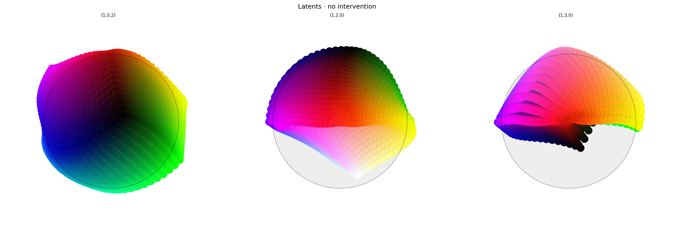
The looks reasonable: similar to Ex 1.7, the latent space shows a color wheel in the first two axes with red near the top. It looks lumpier than I expected, which may mess with the interventions, since they expect unit norm embeddings.
Suppression
Now that we have our model, let's try suppressing red. We'll use the Suppression function developed in Ex 2.1.
from math import pi

import torch

from ex_color.intervention import BoundedFalloff, InterventionConfig, Suppression
from ex_color.vis import plot_colors, plot_cube_series


suppression = Suppression(
    torch.tensor(RED, dtype=torch.float32),  # Constant!
    BoundedFalloff(
        0,  # within 60°
        1,  # completely squash fully-aligned vectors
        2,  # soft rim, sharp hub
    ),
)

interventions = [InterventionConfig(suppression, ['encoder'])]
y_hsv = await infer(model, interventions, x_hsv)
hd_y_hsv = await infer(model, interventions, hd_x_hsv)
clear_output()

with displayer_mpl(
    f'large-assets/ex-{nbid}-pred-colors-suppression.png',
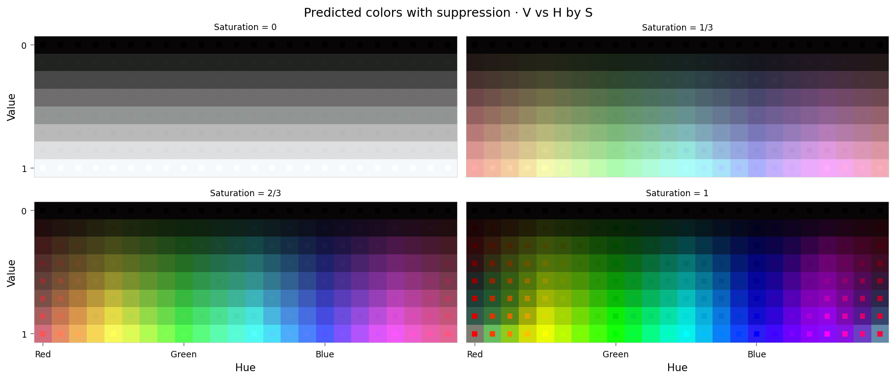
    alt_text="""Plot showing four slices of the HSV cube, titled "Predicted colors with suppression - HSV as H,V per S". Nominally, each slice has constant saturation, but varies in value (brightness) from top to bottom, and in hue from left to right. Each color value is represented as a square patch of that color. The outer portion of the patches shows the color as reconstructed by the model; the inner portion shows the true (input) color. The reconstructed and true colors agree fairly well, but "red" and nearby colors are clearly different: red itself appears as middle-gray, and the surrounding colors up to orange and pink look washed out. "Red-orange" actually appears to be green, moreso even than yellow (which is geometrically closer to green).""",
) as show:
    show(
        lambda: plot_colors(
            hsv_cube,
            title='Predicted colors with suppression',
            colors=y_hsv.numpy(),
            colors_compare=x_hsv.numpy(),
        )
    )

per_color_loss = F.mse_loss(hd_y_hsv, hd_x_hsv, reduction='none').mean(dim=-1)
loss_cube = hd_hsv_cube.assign('MSE', per_color_loss.numpy().reshape(hd_hsv_cube.shape))
max_loss = per_color_loss.max().item()
with displayer_mpl(
    f'large-assets/ex-{nbid}-loss-colors-suppression.png',
    alt_text=f"""Line chart showing loss per color, for colors reconstructed by the model with suppression of red. Y-axis: mean square error, ranging from zero to {max_loss:.2g}. X-axis: hue. There is a significant peak at red at either end of the X-axis, sloping down like a bell curve to low values near yellow and blue. Two small peaks are at blue and pink, with the one at pink around one third the height of the peaks at red.""",
) as show:
    show(
        lambda: plot_cube_series(
            loss_cube.permute('hsv')[:, -1:, :: (loss_cube.shape[2] // -5)],
            loss_cube.permute('svh')[:, -1:, :: -(loss_cube.shape[0] // -6)],
            loss_cube.permute('vsh')[:, -1:, :: -(loss_cube.shape[0] // -6)],
            title='Reconstruction error · suppression',
            var='MSE',
            figsize=(12, 3),
        )
    )
print(f'Max MSE: {max_loss:.2g}')

Max MSE: 0.28
Good! The colors near red have been perturbed, with the effect diminishing on approach to black, yellow, and hot pink.
from IPython.display import clear_output

from ex_color.vis import plot_latent_grid_3d, ConicalAnnotation

y_rgb, h_rgb = await infer_with_latent_capture(model, interventions, x_rgb, 'encoder')
clear_output()

with displayer_mpl(
    f'large-assets/ex-{nbid}-latents-suppression.png',
    alt_text="""Three spherical plots, titled "Latents - suppression". Each plot shows a vibrant collection of colored circles or balls scattered over the surface of a black sphere. The first plot has the appearance of a partial color wheel, with  vibrant colors around the rim (like a rainbow), with with a conspicuously absent space at the top where "red" should be. The other plots show different views of the same sphere, with hue varying across the equator and tone varying from top to bottom, and warm-but-not-red colors in the center (where "red" should be). Each ball shows the reconstructed color, with a dot in the center showing the true (input) color. The true and reconstructor colors agree fairly well, even for the warmer colors. "Red" and nearby colors are in fact not visible, being buried somewhere inside the sphere.""",
) as show:
    show(
        lambda theme: plot_latent_grid_3d(
            h_rgb,
            y_rgb,
            x_rgb,
            title='Latents · suppression',
            dims=[(1, 0, 2), (1, 2, 0), (1, 3, 0)],
            dot_radius=10,
            theme=theme,
            annotations=[
                ConicalAnnotation(
                    RED,
                    2 * (np.pi / 2 - suppression.falloff.a),  # type: ignore
                    color=theme.val('black', dark='#fffa'),
                    linewidth=theme.val(0.5, dark=1),
                    dashes=theme.val((8, 8), dark=(4, 4)),
                    gapcolor=theme.val('#fff4', dark='#0004'),
                ),
            ],
        )
    )
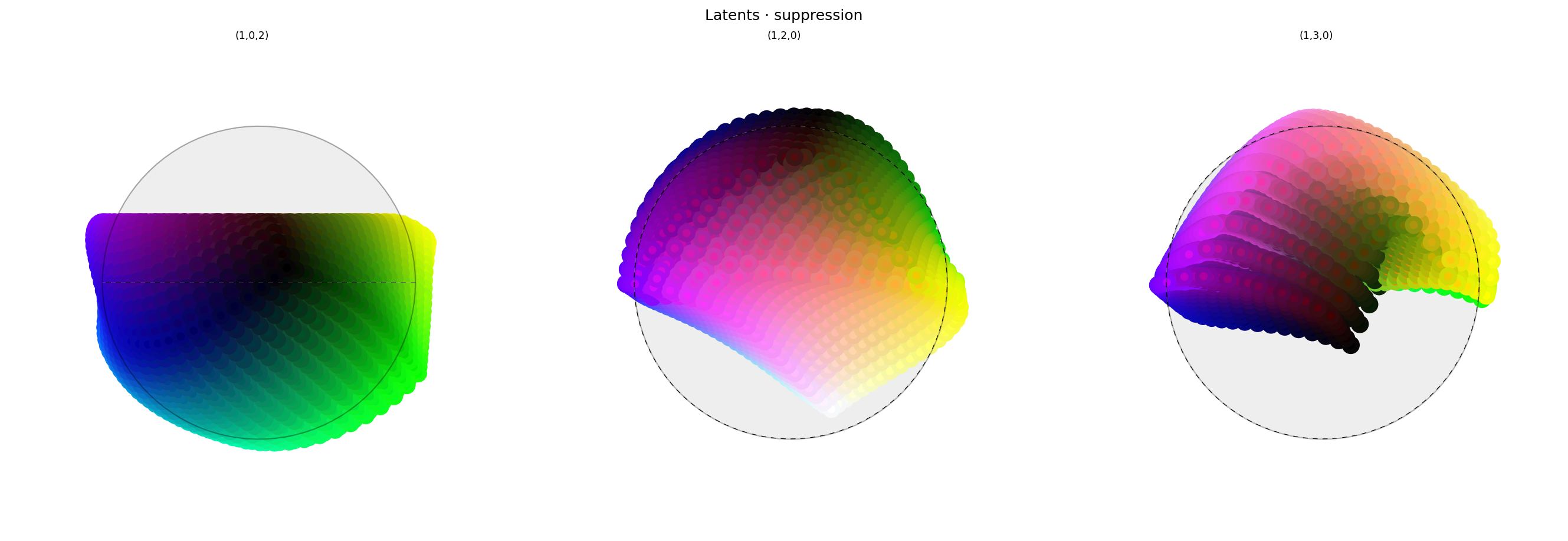
Wow! The way the top of the first plot has been squashed in looks just like the lobe plots from Ex 2.1.
The plots on the right show the same data but looking head-on into the concept vector for red. In the original plots, the centres of these were red. It seems that red has been pushed inside the sphere and is being obscured by other points, so it's a little hard to see what's going on. But we can see from the cube slices above that the model has indeed had its capability to express red interfered with.
It's worth noting that the interior of the sphere is out of distribution from the perspective of the decoder (i.e. downstream from these latents). That's not great, because it should mean the behavior resulting from this intervention is poorly defined.
from math import cos, pi

import torch

from ex_color.intervention import FastBezierMapper, InterventionConfig, Repulsion
from ex_color.vis import plot_colors, plot_cube_series

repulsion = Repulsion(
    torch.tensor([1, 0, 0, 0], dtype=torch.float32),  # Constant!
    FastBezierMapper(
        0,  # Constrain effect to within 60° cone
        cos(pi / 3),  # Create 30° hole (negative cone) around concept vector
    ),
)


interventions = [InterventionConfig(repulsion, ['encoder'])]
y_hsv = await infer(model, interventions, x_hsv)
hd_y_hsv = await infer(model, interventions, hd_x_hsv)
clear_output()

with displayer_mpl(
    f'large-assets/ex-{nbid}-pred-colors-repulsion.png',
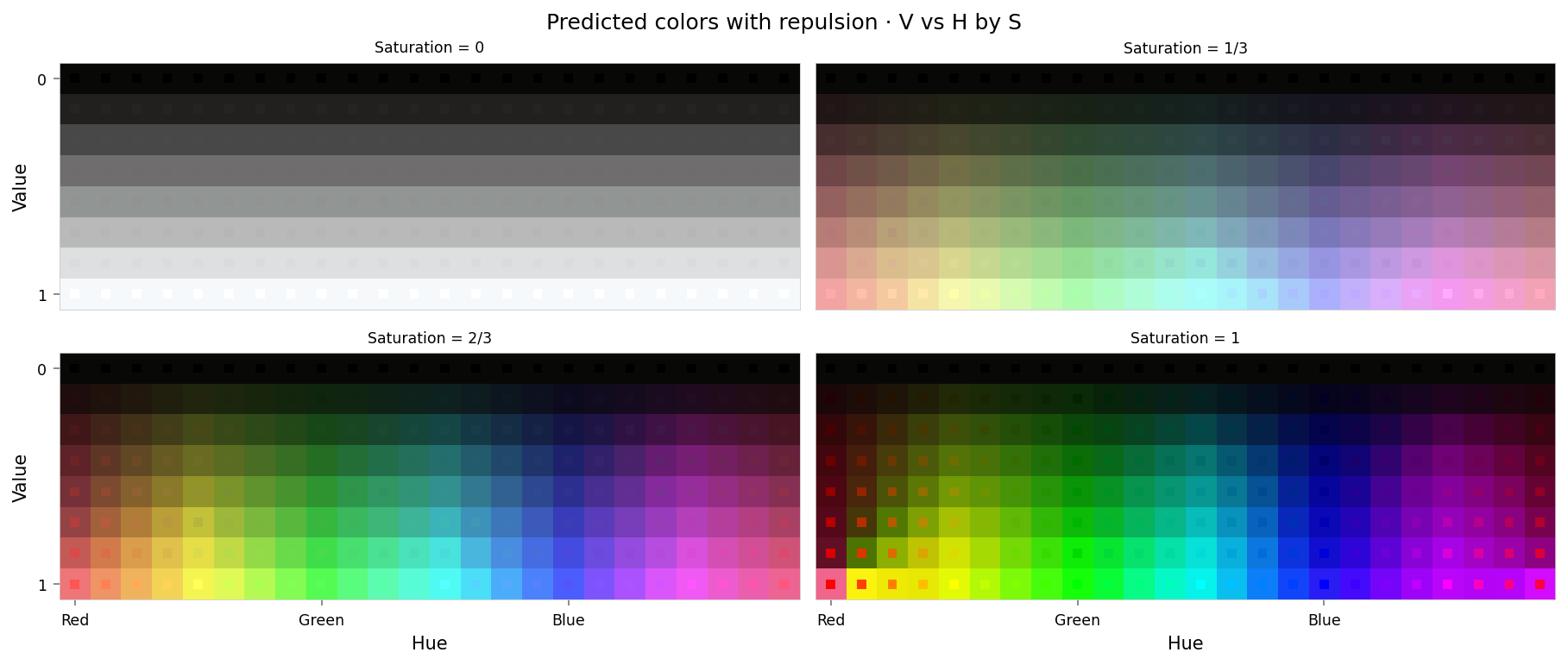
    alt_text="""Plot showing four slices of the HSV cube, titled "Predicted colors with repulsion - HSV as H,V per S". Nominally, each slice has constant saturation, but varies in value (brightness) from top to bottom, and in hue from left to right. Each color value is represented as a square patch of that color. The outer portion of the patches shows the color as reconstructed by the model; the inner portion shows the true (input) color. The reconstructed and true colors agree fairly well, but "red" and nearby colors are clearly different, and different again from how the suppression intervention looked: "red" itself appears as pink or hot pink, and the surrounding colors up to orange and pink look shifted. "Red-orange" actually appears to be fully-saturated yellow. Overall the effect is as though the nearby colors have bled into the neighborhood of red.""",
) as show:
    show(
        lambda: plot_colors(
            hsv_cube,
            title='Predicted colors with repulsion',
            colors=y_hsv.numpy(),
            colors_compare=x_hsv.numpy(),
        )
    )


per_color_loss = F.mse_loss(hd_y_hsv, hd_x_hsv, reduction='none').mean(dim=-1)
loss_cube = hd_hsv_cube.assign('MSE', per_color_loss.numpy().reshape(hd_hsv_cube.shape))
max_loss = per_color_loss.max().item()
with displayer_mpl(
    f'large-assets/ex-{nbid}-loss-colors-repulsion.png',
    alt_text=f"""Line chart showing loss per color, for colors reconstructed by the model with repulsion from red. Y-axis: mean square error, ranging from zero to {max_loss:.2g}. X-axis: hue. There is a significant peak at red at either end of the X-axis, gradually sloping down to lower loss values near yellow and pink. Two very small peaks are at green and blue (apparently around 1% of the height of the peaks at red).""",
) as show:
    show(
        lambda: plot_cube_series(
            loss_cube.permute('hsv')[:, -1:, :: (loss_cube.shape[2] // -5)],
            loss_cube.permute('svh')[:, -1:, :: -(loss_cube.shape[0] // -6)],
            loss_cube.permute('vsh')[:, -1:, :: -(loss_cube.shape[0] // -6)],
            title='Reconstruction error · repulsion',
            var='MSE',
            figsize=(12, 3),
        )
    )
print(f'Max MSE: {max_loss:.2g}')

Max MSE: 0.29
I think this looks quite a lot better than the suppression result: red has been perturbed again, but this time it seems to have been pushed to nearby colors rather than the murky grays we saw previously — so this method seems to preserve more model behavior that we didn't intend to intervene on.
from IPython.display import clear_output

from ex_color.vis import plot_latent_grid_3d, ConicalAnnotation

y_rgb, h_rgb = await infer_with_latent_capture(model, interventions, x_rgb, 'encoder')
clear_output()

with displayer_mpl(
    f'large-assets/ex-{nbid}-latents-repulsion.png',
    alt_text="""Three spherical plots, titled "Latents - repulsion". Each plot shows a vibrant collection of colored circles or balls scattered over the surface of a black sphere. The first plot has the appearance of a partial color wheel, with  vibrant colors around the rim (like a rainbow), with with a conspicuously absent space at the top where "red" should be. The other plots show different views of the same sphere, with hue varying across the equator and tone varying from top to bottom. The central region of the second and third plots show something interesting: "Red" and nearby colors have been arranged into a wide ring or disc, rather than being clustered in the center. Each ball shows the reconstructed color, with a dot in the center showing the true (input) color. The true and reconstructor colors agree fairly well, except for colors close to "red", which roughly agree in saturation but differ significantly in tone and hue.""",
) as show:
    show(
        lambda theme: plot_latent_grid_3d(
            h_rgb,
            y_rgb,
            x_rgb,
            title='Latents · repulsion',
            dims=[(1, 0, 2), (1, 2, 0), (1, 3, 0)],
            dot_radius=10,
            theme=theme,
            annotations=[
                ConicalAnnotation(
                    RED,
                    2 * (np.pi / 2 - repulsion.mapper.a),  # type: ignore
                    color=theme.val('black', dark='#fffa'),
                    linewidth=theme.val(0.5, dark=1),
                    dashes=theme.val((8, 8), dark=(4, 4)),
                    gapcolor=theme.val('#fff4', dark='#0004'),
                ),
                ConicalAnnotation(
                    RED,
                    2 * (np.pi / 2 - repulsion.mapper.b),  # type: ignore
                    color=theme.val('black', dark='#fffa'),
                    linewidth=theme.val(0.5, dark=1),
                ),
            ],
        )
    )
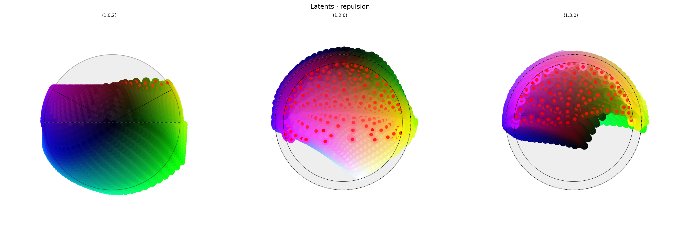
Here we see that the reds have all been pushed away from the intervened-on concept vector, and have formed a ring around it. The two plots on the right show that the points have not been pushed into the sphere interior, which means they're more likely to still be in-distrubtion from the point of view of the decoder. However, the pre-intervention hypersphere isn't covered with points — if our intervention has pushed points into a previously empty region, that would still count as being out of distribution.
Conclusion
Our hypothesis was largely confirmed: the interventions were able to increase the reconstruction loss for colors near red without affecting untargeted colors.
Next steps
Next I'd like to see if the results can be improved by including an explicit normalization step in the forward pass, so that we're not entirely relying on the regularization to shape the embeddings. I expect that will improve both color reconstruction and intervention effectiveness.