Experiment 1.7: Sparse labels (per-sample regularization)

In previous experiments, we imposed structure on latent space with curriculum learning: varying the training data and hyperparameters over the course of the training run (Ex 1.3, Ex 1.5, Ex 1.6). It worked (in that the latent space looked ok), but we are unsure whether it worked because the color wheel was found and anchored before expanding the data to include all colors (i.e. due to the curriculum), or whether it was just that the primary and secondary colors were regularized differently.

In this experiment, we do away with the phased data curriculum, and instead apply per-sample regularization. Our hypothesis is that this will in fact outperform the curriculum-based methods, because the model will have access to the data full distribution from the start (limited only by batch size).

We chose color as a domain because it's easy to reason about and visualize. But since our eventual goal is to apply these techniques to LLM training, we should consider how to constrain the labels in a way that could realistically be replicated for text. We assume that:

1. An LLM would be trained with something like internet text
2. Sentiment analysis could be run over it to generate labels — attributes that we care about, such as "malicious", "benign", "honest", etc.
3. Such labelling would not be entirely accurate.

Therefore for this experiment, we will apply the following regigme:

1. An autoencoder trained on a color cube, as an analog for an LLM
2. Certain colors are given labels (e.g. $(1,0,0)=red$)
3. The labelling will be noisy, e.g. $(1,0,0)$ won't always be labelled as $red$, and sometimes other colors close to red will be given that label.

Certain regularizers will be activated based on those labels, e.g. colors labelled $red$ could be penalized for not being embedded at $(1,0,0,0)$.

from __future__ import annotations

import logging
from utils.logging import SimpleLoggingConfig

logging_config = (
    SimpleLoggingConfig()
    .info('notebook', 'utils', 'mini', 'ex_color')
    .error('matplotlib.axes')  # Silence warnings about set_aspect
)
logging_config.apply()

# ID for tagging assets
nbid = '1.7'
# This is the logger for this notebook
log = logging.getLogger(f'notebook.{nbid}')

Model architecture

We use the same simple 2-layer MLP autoencoder with a 4D bottleneck as in previous experiments.

import torch
import torch.nn as nn

E = 4


class ColorMLP(nn.Module):
    def __init__(self):
        super().__init__()
        # RGB input (3D) → hidden layer → bottleneck → hidden layer → RGB output
        self.encoder = nn.Sequential(
            nn.Linear(3, 16),
            nn.GELU(),
            # nn.Linear(16, 16),
            # nn.GELU(),
            nn.Linear(16, E),  # Our critical bottleneck!
        )

        self.decoder = nn.Sequential(
            nn.Linear(E, 16),
            nn.GELU(),
            # nn.Linear(16, 16),
            # nn.GELU(),
            nn.Linear(16, 3),
            nn.Sigmoid(),  # Keep RGB values in [0,1]
        )

    def forward(self, x: torch.Tensor) -> tuple[torch.Tensor, torch.Tensor]:
        # Get our bottleneck representation
        bottleneck = self.encoder(x)

        # Decode back to RGB
        output = self.decoder(bottleneck)
        return output, bottleneck

Training machinery with timeline and events

The train_color_model function orchestrates the training process based on a Timeline derived from the dopesheet. It handles:

• Iterating through training steps.
• Fetching the correct data loader for the current phase.
• Updating hyperparameters (like learning rate and loss weights) smoothly based on the timeline state.
• Calculating the combined loss from reconstruction and various regularizers.
• Executing the optimizer step.
• Emitting events at different points (phase start/end, pre-step, actions like 'anchor', step metrics) to trigger callbacks like plotting, recording, or updating loss terms.

Improvement over Ex 1.6: regularizers are applied with diffent weights for each sample based on the sample labels.

from dataclasses import dataclass
from typing import Protocol, runtime_checkable
from torch import Tensor
import torch.optim as optim

from mini.temporal.timeline import State


@dataclass
class InferenceResult:
    outputs: Tensor
    latents: Tensor

    def detach(self):
        return InferenceResult(self.outputs.detach(), self.latents.detach())

    def clone(self):
        return InferenceResult(self.outputs.clone(), self.latents.clone())

    def cpu(self):
        return InferenceResult(self.outputs.cpu(), self.latents.cpu())


@runtime_checkable
class LossCriterion(Protocol):
    def __call__(self, data: Tensor, res: InferenceResult) -> Tensor: ...


@dataclass
class RegularizerConfig:
    """Configuration for a regularizer, including label affinities."""

    name: str
    """Matched with hyperparameter for weighting"""
    criterion: LossCriterion
    label_affinities: dict[str, float] | None
    """Maps label names to affinity strengths"""


@dataclass(eq=False, frozen=True)
class Event:
    name: str
    step: int
    model: ColorMLP
    timeline_state: State
    optimizer: optim.Optimizer


@dataclass(eq=False, frozen=True)
class PhaseEndEvent(Event):
    validation_data: Tensor
    inference_result: InferenceResult


@dataclass(eq=False, frozen=True)
class StepMetricsEvent(Event):
    """Event carrying metrics calculated during a training step."""

    train_batch: Tensor
    total_loss: float
    losses: dict[str, float]


class EventHandler[T](Protocol):
    def __call__(self, event: T) -> None: ...


class EventBinding[T]:
    """A class to bind events to handlers."""

    def __init__(self, event_name: str):
        self.event_name = event_name
        self.handlers: list[tuple[str, EventHandler[T]]] = []

    def add_handler(self, event_name: str, handler: EventHandler[T]) -> None:
        self.handlers.append((event_name, handler))

    def emit(self, event_name: str, event: T) -> None:
        for name, handler in self.handlers:
            if name == event_name:
                handler(event)


class EventHandlers:
    """A simple event system to allow for custom callbacks."""

    phase_start: EventBinding[Event]
    pre_step: EventBinding[Event]
    action: EventBinding[Event]
    phase_end: EventBinding[PhaseEndEvent]
    step_metrics: EventBinding[StepMetricsEvent]

    def __init__(self):
        self.phase_start = EventBinding[Event]('phase-start')
        self.pre_step = EventBinding[Event]('pre-step')
        self.action = EventBinding[Event]('action')
        self.phase_end = EventBinding[PhaseEndEvent]('phase-end')
        self.step_metrics = EventBinding[StepMetricsEvent]('step-metrics')

Training loop

import random
import numpy as np
from skimage import metrics
import torch
from typing import Iterable, Iterator
from torch.utils.data import DataLoader
import torch.optim as optim

from mini.temporal.dopesheet import Dopesheet
from mini.temporal.timeline import Timeline
from utils.progress import RichProgress


def seed_everything(seed: int):
    """Set seeds for reproducibility."""
    random.seed(seed)
    np.random.seed(seed)
    torch.manual_seed(seed)
    if torch.cuda.is_available():
        torch.cuda.manual_seed_all(seed)
    log.info(f'Global random seed set to {seed}')


def set_deterministic_mode(seed: int):
    """Make experiments reproducible."""
    seed_everything(seed)
    torch.backends.cudnn.deterministic = True
    torch.backends.cudnn.benchmark = False
    log.info('PyTorch set to deterministic mode')


def reiterate[T](it: Iterable[T]) -> Iterator[T]:
    """
    Iterates over an iterable indefinitely.

    When the iterable is exhausted, it starts over from the beginning. Unlike
    `itertools.cycle`, yielded values are not cached — so each iteration may be
    different.
    """
    while True:
        yield from it


def train_color_model(  # noqa: C901
    model: ColorMLP,
    train_loader: DataLoader,
    val_data: Tensor,
    dopesheet: Dopesheet,
    loss_criterion: LossCriterion,
    regularizers: list[RegularizerConfig],
    event_handlers: EventHandlers | None = None,
):
    if event_handlers is None:
        event_handlers = EventHandlers()

    # --- Validate inputs ---
    if 'lr' not in dopesheet.props:
        raise ValueError("Dopesheet must define the 'lr' property column.")
    # --- End Validation ---

    timeline = Timeline(dopesheet)
    optimizer = optim.Adam(model.parameters(), lr=0)
    device = next(model.parameters()).device

    train_data = iter(reiterate(train_loader))

    total_steps = len(timeline)

    with RichProgress(total=total_steps, description='Training Steps') as pbar:
        for step in range(total_steps):
            # Get state *before* advancing timeline for this step's processing
            current_state = timeline.state
            current_phase_name = current_state.phase

            batch_data, batch_labels = next(train_data)
            # Should already be on device
            # batch_data = batch_data.to(device)
            # batch_labels = batch_labels.to(device)

            # --- Event Handling ---
            event_template = {
                'step': step,
                'model': model,
                'timeline_state': current_state,
                'optimizer': optimizer,
            }

            if current_state.is_phase_start:
                event = Event(name=f'phase-start:{current_phase_name}', **event_template)
                event_handlers.phase_start.emit(event.name, event)
                event_handlers.phase_start.emit('phase-start', event)

            for action in current_state.actions:
                event = Event(name=f'action:{action}', **event_template)
                event_handlers.action.emit(event.name, event)
                event_handlers.action.emit('action', event)

            event = Event(name='pre-step', **event_template)
            event_handlers.pre_step.emit('pre-step', event)

            # --- Training Step ---
            # ... (get data, update LR, zero grad, forward pass, calculate loss, backward, step) ...

            current_lr = current_state.props['lr']
            # REF_BATCH_SIZE = 32
            # lr_scale_factor = batch.shape[0] / REF_BATCH_SIZE
            # current_lr = current_lr * lr_scale_factor
            for param_group in optimizer.param_groups:
                param_group['lr'] = current_lr

            optimizer.zero_grad()

            outputs, latents = model(batch_data)
            current_results = InferenceResult(outputs, latents)

            primary_loss = loss_criterion(batch_data, current_results).mean()
            losses = {'recon': primary_loss.item()}
            total_loss = primary_loss
            zeros = torch.tensor(0.0, device=batch_data.device)

            for regularizer in regularizers:
                name = regularizer.name
                criterion = regularizer.criterion

                weight = current_state.props.get(name, 1.0)
                if weight == 0:
                    continue

                if regularizer.label_affinities is not None:
                    # Soft labels that indicate how much effect this regularizer has, based on its affinity with the label
                    label_probs = [
                        batch_labels[k] * v
                        for k, v in regularizer.label_affinities.items()
                        if k in batch_labels  #
                    ]
                    if not label_probs:
                        continue

                    sample_affinities = torch.stack(label_probs, dim=0).sum(dim=0)
                    sample_affinities = torch.clamp(sample_affinities, 0.0, 1.0)
                    if torch.allclose(sample_affinities, zeros):
                        continue
                else:
                    sample_affinities = torch.ones(batch_data.shape[0], device=batch_data.device)

                per_sample_loss = criterion(batch_data, current_results)
                if len(per_sample_loss.shape) == 0:
                    # If the loss is a scalar, we need to expand it to match the batch size
                    per_sample_loss = per_sample_loss.expand(batch_data.shape[0])
                assert per_sample_loss.shape[0] == batch_data.shape[0], f'Loss should be per-sample OR scalar: {name}'

                # Apply sample affinities
                weighted_loss = per_sample_loss * sample_affinities

                # Apply sample importance weights
                # weighted_loss *= batch_weights

                # Calculate mean only over selected samples. If we used torch.mean, it would average over all samples, including those with 0 weight
                term_loss = weighted_loss.sum() / (sample_affinities.sum() + 1e-8)

                losses[name] = term_loss.item()
                if not torch.isfinite(term_loss):
                    log.warning(f'Loss term {name} at step {step} is not finite: {term_loss}')
                    continue
                total_loss += term_loss * weight

            if total_loss > 0:
                total_loss.backward()
                optimizer.step()
            # --- End Training Step ---

            # Emit step metrics event
            step_metrics_event = StepMetricsEvent(
                name='step-metrics',
                **event_template,
                train_batch=batch_data,
                total_loss=total_loss.item(),
                losses=losses,
            )
            event_handlers.step_metrics.emit('step-metrics', step_metrics_event)

            # --- Post-Step Event Handling ---
            if current_state.is_phase_end:
                # Trigger phase-end for the *current* phase
                # validation_data = batch_data
                with torch.no_grad():
                    val_outputs, val_latents = model(val_data.to(device))
                event = PhaseEndEvent(
                    name=f'phase-end:{current_phase_name}',
                    **event_template,
                    validation_data=val_data,
                    inference_result=InferenceResult(val_outputs, val_latents),
                )
                event_handlers.phase_end.emit(event.name, event)
                event_handlers.phase_end.emit('phase-end', event)
            # --- End Event Handling ---

            # Update progress bar
            pbar.update(
                metrics={
                    'PHASE': current_phase_name,
                    'lr': f'{current_lr:.6f}',
                    'loss': f'{total_loss.item():.4f}',
                    **{name: f'{lt:.4f}' for name, lt in losses.items()},
                },
            )

            # Advance timeline *after* processing the current step
            if step < total_steps:  # Avoid stepping past the end
                timeline.step()

    log.info('Training finished!')

Visualization

We define an event handler that periodically draws scatter plots of the latent embeddings.

import matplotlib.pyplot as plt
from matplotlib.patches import Circle
from matplotlib.axes import Axes
import numpy.typing as npt
from torch import Tensor
from IPython.display import HTML

from utils.nb import save_fig


def hide_decorations(ax: Axes, background: bool = True, ticks: bool = True, border: bool = True) -> None:
    """Remove all decorations from the axes."""
    if background:
        ax.patch.set_alpha(0)
    if ticks:
        ax.set_xticks([])
        ax.set_yticks([])
    if border:
        ax.spines['top'].set_visible(False)
        ax.spines['right'].set_visible(False)
        ax.spines['bottom'].set_visible(False)
        ax.spines['left'].set_visible(False)


def draw_latent_slice(
    ax: Axes | tuple[Axes, Axes],  # Axes for background and foreground
    latents: npt.NDArray,
    colors: npt.NDArray,
    dot_size: float = 200,
    clip_on: bool = False,
):
    """Draw a slice of the latent space."""
    assert latents.ndim == 2, 'Latents should be 2D'
    assert latents.shape[1] == 2, 'Latents should have 2 dimensions'

    bg, fg = ax if isinstance(ax, tuple) else (ax, ax)
    return {
        'circ': bg.add_patch(
            Circle((0, 0), 1, fill=True, facecolor='#111', edgecolor='#0000', clip_on=clip_on, zorder=-1)
        ),
        'scatter': fg.scatter(latents[:, 0], latents[:, 1], c=colors, s=dot_size, alpha=0.7, clip_on=clip_on),
    }


def geometric_frame_progression(samples: int, n: int, offset: int = 10) -> npt.NDArray[np.int_]:
    """
    Generate a geometric progression of indices for sampling frames.

    Useful for creating videos of simulations in which there is more detail at the beginning.

    Args:
        samples (int): Number of samples to generate. If larger than n, it will be capped to n.
        n (int): Total number of frames to sample from.
        offset (int): Offset to apply during generation. Increase this to get more samples at the start of short sequences; larger values will result in "flatter" sequences.

    Returns:
        np.ndarray: Array of indices.
    """
    samples = min(samples, n)
    if samples <= 0:
        return np.array([], dtype=int)
    return np.unique(np.geomspace(offset, n + offset, samples, endpoint=False, dtype=int) - offset)


def bezier_frame_progression(
    samples: int,
    n: int,
    cp1: tuple[float, float],
    cp2: tuple[float, float],
    lookup_table_size: int = 200,
) -> npt.NDArray[np.int_]:
    """
    Generate a bezier curve for sampling frames.

    Args:
        samples: Number of samples to generate (inclusive upper bound).
        n: Total number of frames to sample from.
        cp1: Control point 1 (t_in, t_out), e.g. (0, 0) for a linear curve, or (0.42, 0) for a classic ease-in.
        cp2: Control point 2 (t_in, t_out), e.g. (1, 1) for a linear curve, or (0.58, 1) for a classic ease-out.
        lookup_table_size: Number of points to sample on the bezier curve. Higher values will result in smoother curves, but will take longer to compute.
    """
    from matplotlib.bezier import BezierSegment

    if samples <= 0 or n <= 0:
        return np.array([], dtype=int)
    if n == 1:
        return np.array([0], dtype=int)
    control_points = np.array([(0, 0), cp1, cp2, (1, 1)])
    bezier_curve = BezierSegment(control_points)
    t_lookup = np.linspace(0, 1, lookup_table_size)
    points_on_curve = bezier_curve(t_lookup)
    xs = points_on_curve[:, 0]
    ys = points_on_curve[:, 1]
    assert np.all(np.diff(xs) >= 0), 't is not monotonic'

    # Generate linearly spaced input times for sampling our easing function
    t_linear_input = np.linspace(0, 1, samples, endpoint=True)

    # Interpolate to get eased time:
    # For each t_linear_input (our desired "progress through animation"),
    # find the corresponding y-value on the Bézier curve (our "eased progress").
    t_eased = np.interp(t_linear_input, xs, ys)

    # Clip eased time to [0,1] in case control points caused overshoot/undershoot
    # and we want to strictly map to frame indices.
    t_eased = np.clip(t_eased, 0.0, 1.0)

    # Scale to frame indices and ensure they are unique and sorted
    frame_indices = np.round(t_eased * (n - 1)).astype(int)
    unique_indices = np.unique(frame_indices)

    return unique_indices


class PhasePlotter:
    """Event handler to plot latent space at the end of each phase."""

    def __init__(self, val_data: Tensor, *, dim_pairs: list[tuple[int, int]], interval: int = 100):
        from utils.nb import displayer

        # Store (phase_name, end_step, data, result) - data comes from event now
        self.val_data = val_data
        self.history: list[tuple[str, int, Tensor, Tensor]] = []
        self.display = displayer()
        self.dim_pairs = dim_pairs
        self.interval = interval

    def __call__(self, event: Event):
        # TODO: Don't assume device = CPU
        # TODO: Split this class so that the event handler is separate from the plotting, and so the plotting can happen locally with @run.hither
        if event.step % self.interval != 0:
            return
        phase_name = event.timeline_state.phase
        step = event.step
        output, latents = event.model(self.val_data)

        log.debug(f'Plotting end of phase: {phase_name} at step {step} using provided results.')

        # Append to history
        self.history.append((phase_name, step, output.detach().cpu(), latents.detach().cpu()))

        # Plotting logic remains the same as it already expected CPU tensors
        fig = self._plot_phase_history()
        self.display(
            HTML(
                save_fig(
                    fig,
                    f'large-assets/ex-{nbid}-color-phase-history.png',
                    alt_text='Visualizations of latent space at the end of each curriculum phase.',
                )
            )
        )

    def _plot_phase_history(self):
        if not self.history:
            fig, ax = plt.subplots()
            fig.set_facecolor('#333')
            ax.set_facecolor('#222')
            ax.text(0.5, 0.5, 'Waiting...', ha='center', va='center')
            return fig

        plt.style.use('dark_background')

        # Number of dimension pairs
        num_dim_pairs = len(self.dim_pairs)

        # Cap the number of thumbnails to a maximum for readability
        max_thumbnails = 10
        indices = geometric_frame_progression(max_thumbnails, len(self.history), offset=10)
        history_to_show = [self.history[i] for i in indices]

        # Create figure with gridspec for flexible layout
        fig = plt.figure(figsize=(12, 5), facecolor='#333')

        # Create two separate gridspecs - one for thumbnails, one for latest state
        gs = fig.add_gridspec(2, 1, hspace=0.1, height_ratios=[4, 1])

        # Thumbnail gridspec (bottom row) - only first dimension pair
        # Remove spacing between thumbnails by setting wspace=0
        thumbnail_gs = gs[1].subgridspec(2, max_thumbnails, wspace=0, hspace=0.1, height_ratios=[1, 0])

        # Latest state gridspec (top row) - all dimension pairs
        latest_gs = gs[0].subgridspec(2, num_dim_pairs, wspace=0, hspace=0.1, height_ratios=[0, 1])

        # Get the data
        _colors = self.val_data.numpy()

        # Create thumbnail axes and plot history
        for i, (_, step, _, latents) in enumerate(history_to_show):
            _latents = latents.numpy()

            # Only plot the first dimension pair for thumbnails
            dim1, dim2 = self.dim_pairs[0]

            # Create title for the thumbnail as its own axes, so that it's aligned with the other titles
            axt = fig.add_subplot(thumbnail_gs[1, i])
            axt.text(
                0,
                0,
                f'{step}',
                # transform=axt.transAxes,
                horizontalalignment='center',
                verticalalignment='top',
                fontsize=7,
            )
            # Remove all decorations
            hide_decorations(axt)

            # Create thumbnail axis
            ax = fig.add_subplot(thumbnail_gs[0, i])
            ax.sharex(axt)
            draw_latent_slice(ax, _latents[:, [dim1, dim2]], _colors, dot_size=20)
            hide_decorations(ax)

            # Ensure square aspect ratio
            ax.set_aspect('equal')
            ax.set_adjustable('box')

        # Plot latest state
        # Get the latest data
        phase_name, step, output, latents = self.history[-1]
        _latents = latents.numpy()

        prev_ax = None
        for i, (dim1, dim2) in enumerate(self.dim_pairs):
            # Create title for the thumbnail as its own axes, so that it's aligned with the other titles
            axt = fig.add_subplot(latest_gs[0, i])
            axt.text(
                0,
                0,
                f'[{dim1}, {dim2}]',
                # transform=axt.transAxes,
                horizontalalignment='center',
                fontsize=10,
            )
            hide_decorations(axt)

            # Plot
            ax = fig.add_subplot(latest_gs[1, i])
            ax.sharex(axt)
            if prev_ax is not None:
                ax.sharey(prev_ax)
            prev_ax = ax
            draw_latent_slice(ax, _latents[:, [dim1, dim2]], _colors)
            hide_decorations(ax)

            # Ensure square aspect ratio
            ax.set_aspect('equal')
            ax.set_adjustable('box')

        # Add overall title
        fig.suptitle(f'Latent space — step {step}', fontsize=12, color='white')

        # Use subplots_adjust instead of tight_layout to avoid warnings
        fig.subplots_adjust(top=0.9, bottom=0.1, left=0.1, right=0.95)

        return fig

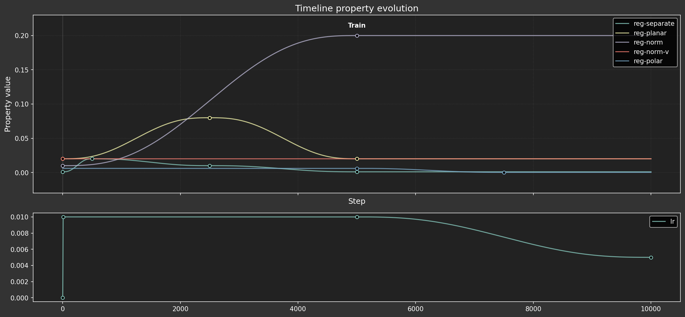
Hyperparameter dopesheet

As in previous experiments, we'll define a dopesheet (timelines) to allow hyperparameters to vary over time. We tried to train the model with constant hyperparameters, but it was difficult to get the training to be stable.

Unlike previous experiments, this one has only one phase, because the full training dataset is used throughout.

import re

from IPython.display import display, HTML
from matplotlib.figure import Figure

from mini.temporal.vis import plot_timeline, realize_timeline, ParamGroup
from mini.temporal.dopesheet import Dopesheet
from mini.temporal.timeline import Timeline
from utils.nb import save_fig


line_styles = [
    (re.compile(r'^data-'), {'linewidth': 5, 'zorder': -1, 'alpha': 0.5}),
    # (re.compile(r'-(anchor|norm)$'), {'linewidth': 2, 'linestyle': (0, (8, 1, 1, 1))}),
]


def load_dopesheet():
    dopesheet = Dopesheet.from_csv(f'ex-{nbid}-dopesheet.csv')
    # display(Markdown(f"""## Parameter schedule ({variant})\n{dopesheet.to_markdown()}"""))

    timeline = Timeline(dopesheet)
    history_df = realize_timeline(timeline)
    keyframes_df = dopesheet.as_df()

    groups = (
        ParamGroup(
            name='',
            params=[p for p in dopesheet.props if p not in {'lr'}],
            height_ratio=2,
        ),
        ParamGroup(
            name='',
            params=[p for p in dopesheet.props if p in {'lr'}],
            height_ratio=1,
        ),
    )
    fig, ax = plot_timeline(history_df, keyframes_df, groups, line_styles=line_styles)
    # Add assertion to satisfy type checker
    assert isinstance(fig, Figure), 'plot_timeline should return a Figure'
    display(
        HTML(
            save_fig(
                fig,
                f'large-assets/ex-{nbid}-color-timeline.png',
                alt_text='Line chart showing the hyperparameter schedule over time.',
            )
        )
    )
    return dopesheet


dopesheet = load_dopesheet()

Loss functions and regularizers

Like Ex 1.6, we use mean squared error for the main reconstruction loss (loss-recon), and regularizers that encourage embeddings of unit length, and for primary colors to be on the plane of the first two dimensions. However this time, the regularizers can have different strengths depending on which sample they're evaluating. See Labelling and Train below.

from torch import linalg as LA

from ex_color.data.color_cube import ColorCube
from ex_color.data.cyclic import arange_cyclic


def objective(fn):
    """Adapt loss function to look like a regularizer"""

    def wrapper(data: Tensor, res: InferenceResult) -> Tensor:
        loss = fn(data, res.outputs)
        # Reduce element-wise loss to per-sample loss by averaging over feature dimensions
        if loss.ndim > 1:
            # Calculate mean over all dimensions except the first (batch) dimension
            reduce_dims = tuple(range(1, loss.ndim))
            loss = torch.mean(loss, dim=reduce_dims)
        return loss

    return wrapper


def unitarity(data: Tensor, res: InferenceResult) -> Tensor:
    """Regularize latents to have unit norm (vectors of length 1)"""
    norms = LA.vector_norm(res.latents, dim=-1)
    # Return per-sample loss, shape [B]
    return (norms - 1.0) ** 2


def planarity(data: Tensor, res: InferenceResult) -> Tensor:
    """Regularize latents to be planar in the first two channels (so zero in other channels)"""
    if res.latents.shape[1] <= 2:
        # No dimensions beyond the first two, return zero loss per sample
        return torch.zeros(res.latents.shape[0], device=res.latents.device)
    # Sum squares across the extra dimensions for each sample, shape [B]
    return torch.sum(res.latents[:, 2:] ** 2, dim=-1)

Pin (anchor)

In Ex 1.5, we used concept anchoring for the primary and secondary colors from the end of the first phase. This time, we'll associate some colors with specific points in latent space right from the start.

The Pin function penalizes points for being far from the chosen location. By itself it would act on all points equally. We tell it which points to apply to when we configure the regularizers (see Train).

class Pin(LossCriterion):
    def __init__(self, anchor_point: Tensor):
        self.anchor_point = anchor_point

    def __call__(self, data: Tensor, res: InferenceResult) -> Tensor:
        """
        Regularize latents to be close to the anchor point.

        Returns:
            loss: Per-sample loss, shape [B].
        """
        # Calculate squared distances to the anchor
        sq_dists = torch.sum((res.latents - self.anchor_point) ** 2, dim=-1)  # [B]
        return sq_dists

Separate

Another regularization term encourages the embeddings to have unit length, but by default, that causes them to bunch up. The Separate function counters that. A similar function was used in Ex 1.5 and 1.6, but it applied a linear (Euclidean) repulsion term — which fought against the unit length normalization. Instead, this one uses cosine similarity to create a repulsive force along the surface of the hypersphere. Since that's orthogonal to the normalization term, they no longer fight against each other.

from types import EllipsisType


class Separate(LossCriterion):
    """Regularize latents to be rotationally separated from each other."""

    def __init__(self, channels: tuple[int, ...] | EllipsisType = ..., power: float = 1.0, shift: bool = True):
        self.channels = channels
        self.power = power
        self.shift = shift

    def __call__(self, data: Tensor, res: InferenceResult) -> Tensor:
        embeddings = res.latents[:, self.channels]  # [B, C]

        # Normalize to unit hypersphere, so it's only the angular distance that matters
        embeddings = embeddings / (torch.norm(embeddings, dim=-1, keepdim=True) + 1e-8)

        # Find the angular distance as cosine similarity
        cos_sim = torch.matmul(embeddings, embeddings.T)  # [B, B]

        # Nullify self-repulsion.
        # We can't use torch.eye, because some points in the batch may be duplicates due to the use of random sampling with replacement.
        cos_sim[torch.isclose(cos_sim, torch.ones_like(cos_sim))] = 0.0
        if self.shift:
            # Shift the cosine similarity to be in the range [0, 1]
            cos_sim = (cos_sim + 1.0) / 2.0

        # Sum over all other points
        return torch.sum(cos_sim**self.power, dim=-1)  # [B]

Data loading, sampling, and event handling

Here we set up:

• Datasets: Define the datasets used (primary/secondary colors, full color grid).
• Sampler: Use DynamicWeightedRandomBatchSampler for the full dataset. Its weights are updated by the update_sampler_weights callback, which responds to the data-fraction parameter from the dopesheet. This smoothly shifts the sampling focus from highly vibrant colors early on to the full range of colors later.
• Recorders: ModelRecorder and MetricsRecorder are event handlers that save the model state and loss values at each step.
• Event bindings: Connect event handlers to specific events (e.g., plotter to phase-end, reg_anchor.on_anchor to action:anchor, recorders to pre-step and step-metrics).
• Training execution: Finally, call train_color_model with the model, datasets, dopesheet, loss criteria, and configured event handlers.

Recorders

import numpy as np
import torch.nn as nn


class ModelRecorder(EventHandler):
    """Event handler to record model parameters."""

    history: list[tuple[int, dict[str, Tensor]]]
    """A list of tuples (step, state_dict) where state_dict is a copy of the model's state dict."""

    def __init__(self):
        self.history = []

    def __call__(self, event: Event):
        # Get a *copy* of the state dict and move it to the CPU
        # so we don't hold onto GPU memory or track gradients unnecessarily.
        model_state = {k: v.cpu().clone() for k, v in event.model.state_dict().items()}
        self.history.append((event.step, model_state))
        log.debug(f'Recorded model state at step {event.step}')


class BatchRecorder(EventHandler):
    """Event handler to record the exact batches used at each step."""

    history: list[tuple[int, Tensor]]
    """A list of tuples (step, train_batch)."""

    def __init__(self):
        self.history = []

    def __call__(self, event: StepMetricsEvent):
        if not isinstance(event, StepMetricsEvent):
            log.warning(f'BatchRecorder received unexpected event type: {type(event)}')
            return
        self.history.append((event.step, event.train_batch.cpu().clone()))
        log.debug(f'Recorded batch at step {event.step}')


class MetricsRecorder(EventHandler):
    """Event handler to record training metrics."""

    history: list[tuple[int, float, dict[str, float]]]
    """A list of tuples (step, total_loss, losses_dict)."""

    def __init__(self):
        self.history = []

    def __call__(self, event: StepMetricsEvent):
        if not isinstance(event, StepMetricsEvent):
            log.warning(f'MetricsRecorder received unexpected event type: {type(event)}')
            return

        self.history.append((event.step, event.total_loss, event.losses.copy()))
        log.debug(f'Recorded metrics at step {event.step}: loss={event.total_loss:.4f}')

Labelling

The training dataset has a fixed and somewhat small size. We want to simulate noisy labels — e.g. RGB 1,0,0 should not always be labelled "red", and colors close to red should also sometimes attract that label.

Here we define a collation function for use with DataLoader. It takes a batch and produces labels for the samples on the fly, which means the model may see identical samples with different labels during training.

Labels are assigned based on proximity to certain colors. The raw distance is not used; instead it is raised to a power to sharpen the association, and weaken the label for colors that are futher away. Initially the labels are smooth $(0..1)$. They are then converted to binary $\lbrace 0,1 \rbrace$ by comparison to random numbers.

The label "red" (i.e. proximity to pure red) is calculated as:

$$\text{red} = \left(r - \frac{rg}{2} - \frac{rb}{2}\right) ^{10}$$

While "vibrant" (proximity to any pure hue) is:

$$\text{vibrant} = \left(s \times v\right)^{100}$$

Where $r$, $g$, and $b$ are the red, green, and blue channels, and $s$ and $v$ are the saturation and value — all of which are real numbers between 0 and 1.

import torch
from torch.utils.data import DataLoader, TensorDataset, WeightedRandomSampler
from torch.utils.data.dataloader import default_collate

# TODO: remove forced reload
if True:
    import importlib
    import ex_color.data.cube_sampler

    importlib.reload(ex_color.data.cube_sampler)


def generate_color_labels(data: Tensor, vibrancies: Tensor) -> dict[str, Tensor]:
    """
    Generate label probabilities based on RGB values.

    Args:
        data: Batch of RGB values [B, 3]

    Returns:
        Dictionary mapping label names to probabilities str -> [B]
    """
    labels: dict[str, Tensor] = {}

    # Labels are assigned based on proximity to certain colors.
    # Distance is raised to a power to sharpen the association (i.e. weaken the label for colors that are futher away).

    # Proximity to primary colors
    r, g, b = data[:, 0], data[:, 1], data[:, 2]
    labels['red'] = (r * (1 - g / 2 - b / 2)) ** 10
    # labels['green'] = g * (1 - r / 2 - b / 2)
    # labels['blue'] = b * (1 - r / 2 - g / 2)

    # Proximity to any fully-saturated, fully-bright color
    labels['vibrant'] = vibrancies**100

    return labels


def collate_with_generated_labels(
    batch,
    *,
    soft: bool = True,
    scale: dict[str, float] | None = None,
) -> tuple[Tensor, dict[str, Tensor]]:
    """
    Custom collate function that generates labels for the samples.

    Args:
        batch: A list of ((data_tensor,), index_tensor) tuples from TensorDataset.
               Note: TensorDataset wraps single tensors in a tuple.
        soft: If True, return soft labels (0..1). Otherwise, return hard labels (0 or 1).
        scale: Linear scaling factors for the labels (applied before discretizing).

    Returns:
        A tuple: (collated_data_tensor, collated_labels_tensor)
    """
    # Separate data and indices
    # TensorDataset yields tuples like ((data_point_tensor,), index_scalar_tensor)
    data_tuple_list = [item[0] for item in batch]  # List of (data_tensor,) tuples
    vibrancies = [item[1] for item in batch]

    # Collate the data points using the default collate function
    # default_collate handles the list of (data_tensor,) tuples correctly
    collated_data = default_collate(data_tuple_list)
    vibrancies = default_collate(vibrancies)
    label_probs = generate_color_labels(collated_data, vibrancies)
    for k, v in (scale or {}).items():
        label_probs[k] = label_probs[k] * v

    if soft:
        # Return the probabilities directly
        return collated_data, label_probs
    else:
        # Sample labels stochastically
        labels = {k: discretize(v) for k, v in label_probs.items()}
        return collated_data, labels


def discretize(probs: Tensor) -> Tensor:
    """
    Discretize probabilities into binary labels.

    Args:
        probs: Tensor of probabilities [B]

    Returns:
        Tensor of binary labels [B]
    """
    # Sample from a uniform distribution
    rand = torch.rand_like(probs)
    return (rand < probs).float()  # Convert to float for compatibility with loss functions

Datasets

Like Ex 1.5, we'll train on the HSV cube (with RGB values) and validate with the RGB cube. Unlike Ex 1.5, we don't define a special dataset for the primary and secondary colors. And unlike Ex 1.6, we don't start with a subset of the training data: we train on the whole HSV cube, right from the start. We still use a sampling bias to prevent over-sampling of dark and desaturated colors, but it's held constant throughout training.

from functools import partial
from ex_color.data.cube_sampler import vibrancy

hsv_cube = ColorCube.from_hsv(
    h=arange_cyclic(step_size=10 / 360),
    s=np.linspace(0, 1, 10),
    v=np.linspace(0, 1, 10),
)
hsv_tensor = torch.tensor(hsv_cube.rgb_grid.reshape(-1, 3), dtype=torch.float32)
vibrancy_tensor = torch.tensor(vibrancy(hsv_cube).flatten(), dtype=torch.float32)
hsv_dataset = TensorDataset(hsv_tensor, vibrancy_tensor)

labeller = partial(
    collate_with_generated_labels,
    soft=False,  # Use binary labels (stochastic) to simulate the labelling of internet text
    scale={'red': 0.5, 'vibrant': 0.5},
)
# Desaturated and dark colors are over-represented in the cube, so we use a weighted sampler to balance them out
hsv_loader = DataLoader(
    hsv_dataset,
    batch_size=64,
    sampler=WeightedRandomSampler(
        weights=hsv_cube.bias.flatten().tolist(),
        num_samples=len(hsv_dataset),
        replacement=True,
    ),
    collate_fn=labeller,
)

rgb_cube = ColorCube.from_rgb(
    r=np.linspace(0, 1, 8),
    g=np.linspace(0, 1, 8),
    b=np.linspace(0, 1, 8),
)
rgb_tensor = torch.tensor(rgb_cube.rgb_grid.reshape(-1, 3), dtype=torch.float32)

Train

Regularizer configuration

The training process employs several regularizers, each designed to impose specific structural properties on the latent space. The strength of these regularizers can be modulated by hyperparameters defined in the dopesheet, and their application to individual samples can be influenced by per-sample labels.

Here's a breakdown of each configured regularizer:

• reg-polar: Concept anchor for the color red.

  • Criterion: Pin to the latent coordinate (1, 0, 0, 0). This encourages specific embeddings to move towards this "polar" anchor point.
  • Label affinity: {'red': 1.0}. This regularizer is fully active (strength 1.0) for samples that are labeled as 'red'. Its goal is to anchor the concept of "red" to a specific location in the latent space.

• reg-separate: Encourages the full space to be used.

  • Criterion: Separate (with power=10.0, shift=False). This term encourages all embeddings in a batch to be rotationally distinct from each other. It calculates the cosine similarity between embeddings and applies a repulsive force, powered up to make the effect greater for pairs of points that are very close. The shift=False means it uses the raw cosine similarity (ranging from -1 to 1).
  • Label affinity: None. This regularizer applies equally to all samples in the batch, irrespective of their labels, aiming for a general separation of all learned representations.

• reg-planar: Defines a "hue" plane, onto which the color wheel should emerge.

  • Criterion: planarity. This penalizes embeddings for having non-zero values in latent dimensions beyond the first two (i.e., dimensions 2 and 3, given a 4D latent space). It encourages these embeddings to lie on the plane defined by the first two latent dimensions.
  • Label affinity: {'vibrant': 1.0}. This regularizer is fully active for samples labeled as 'vibrant'. The idea is to map vibrant, pure hues primarily onto a 2D manifold within the latent space, potentially representing a color wheel.

• reg-norm-v: Encourages a circular color wheel, rather than hexagonal.

  • Criterion: unitarity. This encourages the latent embeddings to have a norm (length) of 1, pushing them towards the surface of a hypersphere.
  • Label affinity: {'vibrant': 1.0}. This normalization is specifically applied with full strength to samples labeled as 'vibrant'. This works in conjunction with reg-planar to organize vibrant colors on a 2D spherical surface.

• reg-norm: Encourages embeddings to lie on the surface of a hypersphere, so they can be compared with cosine distance alone.

  • Criterion: unitarity. This also encourages latent embeddings to have a unit norm.
  • Label affinity: None. This regularizer applies the unit norm constraint to all samples in the batch, regardless of their labels. This ensures that even non-vibrant colors are normalized, contributing to a more uniform distribution of embeddings on the hypersphere.

def train(dopesheet: Dopesheet):
    """Train the model with the given dopesheet and variant."""
    log.info('Training')
    recorder = ModelRecorder()
    metrics_recorder = MetricsRecorder()
    batch_recorder = BatchRecorder()

    # seed = 0
    # set_deterministic_mode(seed)

    model = ColorMLP()
    total_params = sum(p.numel() for p in model.parameters() if p.requires_grad)
    log.info(f'Model initialized with {total_params:,} trainable parameters.')

    event_handlers = EventHandlers()
    event_handlers.pre_step.add_handler('pre-step', recorder)
    event_handlers.step_metrics.add_handler('step-metrics', metrics_recorder)
    event_handlers.step_metrics.add_handler('step-metrics', batch_recorder)

    plotter = PhasePlotter(rgb_tensor, dim_pairs=[(1, 0), (1, 2), (1, 3)], interval=200)
    event_handlers.pre_step.add_handler('pre-step', plotter)

    regularizers = [
        RegularizerConfig(
            name='reg-polar',
            criterion=Pin(torch.tensor([1, 0, 0, 0], dtype=torch.float32, device=hsv_tensor.device)),
            label_affinities={'red': 1.0},
        ),
        RegularizerConfig(
            name='reg-separate',
            criterion=Separate(power=10.0, shift=False),
            label_affinities=None,
        ),
        RegularizerConfig(
            name='reg-planar',
            criterion=planarity,
            label_affinities={'vibrant': 1.0},
        ),
        RegularizerConfig(
            name='reg-norm-v',
            criterion=unitarity,
            label_affinities={'vibrant': 1.0},
        ),
        RegularizerConfig(
            name='reg-norm',
            criterion=unitarity,
            label_affinities=None,
        ),
    ]

    train_color_model(
        model,
        hsv_loader,
        rgb_tensor,
        dopesheet,
        # loss_criterion=objective(nn.MSELoss(reduction='none')),  # No reduction; allows per-sample loss weights
        loss_criterion=objective(nn.MSELoss()),
        regularizers=regularizers,
        event_handlers=event_handlers,
    )

    return recorder, metrics_recorder

recorder, metrics = train(dopesheet)

I 3.1 no.1.7:  Training
I 3.1 no.1.7:  Model initialized with 263 trainable parameters.

Training Steps: 100.0% [10001/10001] [00:54/<00:00, 182.18 it/s]

PHASE

lr

loss

recon

reg-separate

reg-planar

reg-norm-v

reg-norm

Train

0.005000

0.0034

0.0003

2.7890

0.0099

0.0002

0.0006

I 58.7 no.1.7: Training finished!

The model trained well! It's interesting that it starts out with quite a regular shape, and then becomes contorted before settling down to a smooth sphere.

Validation

Latent space evolution analysis

Let's visualize how the latent spaces evolved over time. Like Ex 1.5 and 1.6, we'll use the ModelRecorder's history to load the model state at each recorded step and evaluate the latent positions for a fixed set of input colors (the full RGB grid). This gives us a sequence of latent space snapshots.

import numpy as np


def eval_latent_history(
    recorder: ModelRecorder,
    rgb_tensor: Tensor,
):
    """Evaluate the latent space for each step in the recorder's history."""
    # Create a new model instance
    from utils.progress import RichProgress

    model = ColorMLP()

    latent_history: list[tuple[int, np.ndarray]] = []
    # Iterate over the recorded history
    for step, state_dict in RichProgress(recorder.history, description='Evaluating latents'):
        # Load the model state dict
        model.load_state_dict(state_dict)
        model.eval()
        with torch.no_grad():
            # Get the latents for the RGB tensor
            _, latents = model(rgb_tensor.to(next(model.parameters()).device))
            latents = latents.cpu().numpy()
            latent_history.append((step, latents))
    return latent_history


latent_history = eval_latent_history(recorder, rgb_tensor)

Evaluating latents: 0.0% [0/10001] [00:00/<00:00, 0.00 it/s]

Animation of latent space

This final visualization combines multiple views into a single animation:

• Latent space: Shows 2D projections of the latent embeddings for the full RGB color grid, colored by their true RGB values. Note that these projections were not searched for: we knew where to look because we intentionally structured the latent space.
• Hyperparameters: Plots the parameter schedule from the dopesheet, with a vertical line indicating the current step in the animation.
• Training metrics: Plots the total loss and the contribution of each individual loss/regularization term (on a log scale), again with a vertical line for the current step.

A variable stride is used for sampling frames to focus on periods of rapid change.

Improvements over Ex 1.5 and 1.6:

• Better layout: embedding scatter plots are much more prominent, and show multiple views
• Motion blur: "skipped" frames are all rendered on top of each other to accurately show the motion of the points.

from numpy._typing._array_like import NDArray
import matplotlib.pyplot as plt
import matplotlib.animation as animation
import imageio_ffmpeg
from matplotlib import rcParams
import pandas as pd
from matplotlib.gridspec import GridSpec
from matplotlib.collections import PathCollection
from matplotlib.text import Text
from matplotlib.typing import ColorType

from mini.temporal.dopesheet import RESERVED_COLS
from utils.progress import RichProgress

if True:
    import importlib
    import mini.temporal.vis

    importlib.reload(mini.temporal.vis)
from mini.temporal.vis import group_properties_by_scale, plot_timeline

rcParams['animation.ffmpeg_path'] = imageio_ffmpeg.get_ffmpeg_exe()


def animate_latent_evolution_with_metrics(
    # Data
    sampled_indices: NDArray[np.int_],
    latent_history: list[tuple[int, np.ndarray]],
    metrics_history: list[tuple[int, float, dict[str, float]]],
    param_history_df: pd.DataFrame,
    param_keyframes_df: pd.DataFrame,
    # Settings
    colors: np.ndarray,
    dimensions: list[tuple[str, tuple[int, int]]],  # [D, 2]
    interval=1 / 30,  # FPS
    loss_smooth_window: int = 100,
    alpha=0.7,
):
    """Create an animation of latent space evolution, hyperparameters, and metrics."""
    plt.style.use('dark_background')
    # Aim for 16:9 aspect ratio, give latent plots more height
    fig = plt.figure(figsize=(19.20, 10.80))
    fig.patch.set_facecolor('#333')

    fig.subplots_adjust(
        left=0.05,  # Smaller left margin
        right=0.95,  # Smaller right margin
        bottom=0.08,  # Smaller bottom margin (leave room for x-label)
        top=0.93,  # Smaller top margin (leave room for titles)
    )

    # Top row: Latent space evolution [D]
    # Bottom row: Hyperparameters and metrics [2]
    gs = GridSpec(2, 1, height_ratios=[5, 1], hspace=0)
    latent_gs = gs[0].subgridspec(2, len(dimensions), wspace=0, hspace=0, height_ratios=[0, 1])
    metrics_gs = gs[1].subgridspec(1, 2, wspace=0.1)

    # --- Set up latent space axes, and draw once ---

    axs_latent_title: list[Axes] = [fig.add_subplot(latent_gs[0, i], frameon=False) for i, _ in enumerate(dimensions)]
    add_projection_titles(axs_latent_title, dimensions)

    # With clipping off, the backgrounds will overlap. So, add TWO axes for each dimension pair: one for the background and one for the foreground. Create them up-front to set the stacking order.
    axs_latent_bg: list[Axes] = [
        fig.add_subplot(latent_gs[1, i], frameon=False)
        for i, _ in enumerate(dimensions)  # Stacking doesn't matter for the background
    ]
    axs_latent_fg: list[Axes] = list(reversed([
        fig.add_subplot(latent_gs[1, i], frameon=False)
        for i, _ in reversed(list(enumerate(dimensions)))  # Stack in reverse, so the first one is on top
    ]))  # fmt: skip
    scatters = add_projection_plots(axs_latent_bg, axs_latent_fg, dimensions, colors)

    # Parameter plot
    ax_params = fig.add_subplot(metrics_gs[0])
    param_vline, params_legend = add_parameter_plot(ax_params, param_history_df, param_keyframes_df)

    # Metrics plot
    ax_metrics = fig.add_subplot(metrics_gs[1])
    line_colors = {text.get_text(): text.get_color() for text in params_legend}
    metrics_vline, _ = add_metrics_plot(ax_metrics, metrics_history, 0, loss_smooth_window, line_colors)

    # --- Set common X limits ---
    # Only set xlim for the timeline plots (params and metrics)
    max_step = param_history_df['STEP'].max()
    ax_params.set_xlim(left=0, right=max_step)
    ax_metrics.set_xlim(left=0, right=max_step)

    def update(frame: int):
        i1 = sampled_indices[frame]
        i2 = sampled_indices[frame + 1] if frame + 1 < len(sampled_indices) else i1 + 1
        subframes = latent_history[i1:i2]
        if not subframes:
            return ()
        step, _ = subframes[-1]
        # log.info(f'Step {step} ({i1} -> {i2})')

        # --- MOTION BLUR ---
        # Gather the latents for this frame across all included steps.
        # We want to draw the points in the order [B,S], i.e. the _step_ should vary first, so that subsequent points are drawn on top of previous ones.
        # If the order was [S,B], then all points from later steps would obscure earlier ones.
        _latents = [h[1] for h in subframes]  # [S][B, D]
        _colors = [colors] * len(subframes)  # [S][B, C]
        _latents = np.stack(_latents, axis=1)  # [B, S, D]
        _colors = np.stack(_colors, axis=1)  # [B, S, C]
        _latents = np.reshape(_latents, (-1, _latents.shape[-1]))  # [B*S, D]
        _colors = np.reshape(_colors, (-1, _colors.shape[-1]))  # [B*S, C]
        _alpha = distribute_alpha(alpha, len(subframes))

        for scatter, (_, dim_pair) in zip(scatters, dimensions, strict=True):
            scatter.set_offsets(_latents[:, dim_pair])
            scatter.set_color(_colors[:, :3])  # type: ignore
            scatter.set_alpha(_alpha)

        speed = subframes[-1][0] - subframes[0][0] + 1
        speed_text = f'▸▸{speed}x' if speed > 1 else f' ▸{speed}x'

        fig.suptitle(f'Latent space @ {step} {speed_text}')
        param_vline.set_xdata([step])
        metrics_vline.set_xdata([step])

        # Signal that these artists have changed
        return (param_vline, metrics_vline, *scatters)

    # Use the length of the (potentially strided) latent_history for frames
    num_frames = len(sampled_indices)
    ani = animation.FuncAnimation(fig, update, frames=num_frames, interval=interval * 1000, blit=True)
    return fig, ani


def unobtrusive_legend(ax: Axes):
    """Create a legend that doesn't block the plot."""
    lines = [l for l in ax.get_lines() if l.get_label() and not str(l.get_label()).startswith('_')]
    labels = [str(line.get_label()) for line in lines]
    colors = [line.get_color() for line in lines]
    xs = np.linspace(0, 1, len(labels), endpoint=False)
    xs += 0.5 / len(labels)

    artists: list[Text] = []
    for xpos, label, color in zip(xs, labels, colors, strict=True):
        artist = ax.text(
            xpos,
            0.98,
            label,
            transform=ax.transAxes,
            horizontalalignment='center',
            verticalalignment='top',
            fontsize='small',
            color=color,
        )
        artists.append(artist)
    return artists


def add_projection_titles(axs_latent_title: list[Axes], dimensions: list[tuple[str, tuple[int, int]]]):
    # Titles get their own axes, so they can be aligned with the other titles
    for axt, (label, dim_pair) in zip(axs_latent_title, dimensions, strict=True):
        ax_title = f'[{dim_pair[0]},{dim_pair[1]}]'
        axt.text(
            0.5,
            0,
            f'{ax_title} ({label})' if label else ax_title,
            horizontalalignment='center',
            verticalalignment='top',
            fontsize=12,
            color='white',
            alpha=0.5,
        )
        hide_decorations(axt)


def add_projection_plots(
    axs_latent_bg: list[Axes],
    axs_latent_fg: list[Axes],
    dimensions: list[tuple[str, tuple[int, int]]],
    colors: np.ndarray,
):
    scatters: list[PathCollection] = []
    prev_ax = None
    for ax_bg, ax_fg, (_, dim_pair) in zip(axs_latent_bg, axs_latent_fg, dimensions, strict=True):
        # Draw first frame
        _, _latents = latent_history[0]

        ax_bg.set_aspect('equal', adjustable='datalim')
        ax_fg.set_aspect('equal', adjustable='datalim')
        # ax_bg.sharex(ax_fg)
        ax_bg.sharey(ax_fg)
        if prev_ax:
            ax_fg.sharey(prev_ax)
        ax_bg.set_xlim(-1.5, 1.5)
        ax_bg.set_ylim(-1.5, 1.5)
        ax_fg.set_xlim(-1.5, 1.5)
        ax_fg.set_ylim(-1.5, 1.5)
        hide_decorations(ax_bg)
        hide_decorations(ax_fg)
        M = ax_fg.transData.get_matrix()
        xscale = M[0, 0]
        # yscale = M[1,1]

        _latents = _latents[:, dim_pair]
        scatter = draw_latent_slice((ax_bg, ax_fg), _latents, colors, dot_size=(xscale * 0.2) ** 2, clip_on=False)[
            'scatter'
        ]

        prev_ax = ax_fg
        # ax.patch.set_alpha(1)
        scatters.append(scatter)
    return scatters


def add_parameter_plot(
    ax: Axes,
    param_history_df: pd.DataFrame,
    param_keyframes_df: pd.DataFrame,
):
    ax.patch.set_facecolor('#222')
    ax.tick_params(colors='#aaa')
    hide_decorations(ax, ticks=False, background=False)
    param_props = param_keyframes_df.columns.difference(list(RESERVED_COLS)).tolist()
    param_groups = group_properties_by_scale(param_keyframes_df[param_props])
    plot_timeline(
        param_history_df,
        param_keyframes_df,
        [param_groups[0]],
        ax=ax,
        show_legend=False,
        show_phase_labels=False,
        line_styles=line_styles,
    )
    ax.set_xlabel('Step', fontsize='small')
    ax.set_ylabel('Param value', fontsize='small')
    # ax.set_yscale('log')
    param_vline = ax.axvline(0, color='white', linestyle='--', lw=1)
    params_legend = unobtrusive_legend(ax)
    return param_vline, params_legend


def add_metrics_plot(
    ax: Axes,
    metrics_history: list[tuple[int, float, dict[str, float]]],
    step: int,
    loss_smooth_window: int,
    line_colors: dict[str, ColorType],
):
    ax.patch.set_facecolor('#222')
    ax.yaxis.tick_right()
    ax.yaxis.set_label_position('right')
    ax.tick_params(colors='#aaa')
    hide_decorations(ax, ticks=False, background=False)

    metrics_steps = [h[0] for h in metrics_history]

    loss_components = {
        k: np.array([h[2].get(k, np.nan) for h in metrics_history])  #
        for k in metrics_history[0][2].keys()
    }
    loss_components = {
        k: pd.Series(v).ffill().to_numpy()  #
        for k, v in loss_components.items()
    }
    loss_components = {
        k: np.convolve(v, np.ones(loss_smooth_window) / loss_smooth_window, mode='same')  #
        for k, v in loss_components.items()
    }

    # ax.plot(metrics_steps, total_losses, label='Total Loss', lw=1)
    for name, values in loss_components.items():
        ax.plot(metrics_steps, values, label=name, lw=1, alpha=0.8, color=line_colors.get(name))
    ax.set_xlabel('Step', fontsize='small')
    ax.set_ylabel('Loss', fontsize='small')
    ax.set_yscale('log')
    metrics_vline = ax.axvline(step, color='white', linestyle='--', lw=1)
    metrics_legend = unobtrusive_legend(ax)
    return metrics_vline, metrics_legend


def distribute_alpha(alpha: float, n_subframes: int) -> float:
    """Calculate an alpha value to use for each subframe, such that the perceptual alpha for stationary objects is roughly the same as the original."""
    # Base calculation works well for transparent objects (alpha << 1), but for opaque objects it's too opaque.
    base_alpha = 1 - (1 - alpha) ** (1 / n_subframes)
    opaque_alpha = 0.99 / (1 + np.log(n_subframes))

    opaque_influence = alpha**5  # To make it affect mostly opaque objects
    _alpha = np.interp(opaque_influence, [0, 1], [base_alpha, opaque_alpha])

    log.debug(f'N: {n_subframes:3d} Alpha: {alpha:.2f} -> {_alpha:.2f} (base: {base_alpha:.2f}, opaque: {opaque_alpha:.2f})')  # fmt: skip
    return _alpha


# distribute_alpha(1.0, 1)
# distribute_alpha(1.0, 2)
# distribute_alpha(1.0, 3)
# distribute_alpha(1.0, 10)
# distribute_alpha(1.0, 100)

# distribute_alpha(0.95, 1)
# distribute_alpha(0.95, 2)
# distribute_alpha(0.95, 3)
# distribute_alpha(0.95, 10)
# distribute_alpha(0.95, 100)

# distribute_alpha(0.9, 1)
# distribute_alpha(0.9, 2)
# distribute_alpha(0.9, 3)
# distribute_alpha(0.9, 10)
# distribute_alpha(0.9, 100)

# distribute_alpha(0.5, 1)
# distribute_alpha(0.5, 2)
# distribute_alpha(0.5, 3)
# distribute_alpha(0.5, 10)
# distribute_alpha(0.5, 100)

sampled_indices = bezier_frame_progression(
    1000,
    len(latent_history),
    (0.42, 0.0),  # Ease-in (soft)
    (0.95, 1.0),  # Ease-out (sharp)
)

# sampled_indices = sampled_indices[500:510]  # Limit the number of samples during development
# sampled_indices = sampled_indices[-10:]  # Limit the number of samples during development

steps = [latent_history[i][0] for i in sampled_indices]
delta_steps = np.diff(steps)
# Find out how many frames at the start have the same timestep
n_ease_in_frames = np.argmax(delta_steps != delta_steps[0]) + 1
n_ease_out_frames = np.argmax(delta_steps[::-1] != delta_steps[-1]) + 1
log.info(f'Sampled {len(sampled_indices)} of {len(latent_history)} frames ({steps[0]}..{steps[-1]}).')
log.info(f'Timestep at start: {delta_steps[0]}, for {n_ease_in_frames} frames.')
log.info(f'Largest timestep: {max(delta_steps)}.')
log.info(f'Timestep at end: {delta_steps[-1]}, for {n_ease_out_frames} frames.')

# Realize timelines for both dopesheets
timeline = Timeline(dopesheet)
history_df = realize_timeline(timeline)
keyframes_df = dopesheet.as_df()

# --- Render ---
fig, ani = animate_latent_evolution_with_metrics(
    sampled_indices=sampled_indices,
    latent_history=latent_history,
    metrics_history=metrics.history,
    param_history_df=history_df,
    param_keyframes_df=keyframes_df,
    colors=rgb_tensor.cpu().numpy(),
    dimensions=[('hue', (1, 0)), ('', (1, 2)), ('', (3, 2))],
    loss_smooth_window=25,
    alpha=0.9,
)

# --- Save the video ---
video_file = f'large-assets/ex-{nbid}-latent-evolution.mp4'
step_sizes = np.concatenate((delta_steps, [1]))
with RichProgress(total=len(sampled_indices), description='Rendering video') as pbar:
    ani.save(
        video_file,
        fps=30,
        extra_args=['-vcodec', 'libx264'],
        progress_callback=lambda i, n: pbar.update(1, metrics={'step': sampled_indices[i], 'subframes': step_sizes[i]}),
    )
plt.close(fig)

# --- Display the video ---
import secrets
from IPython.display import display, HTML

cache_buster = secrets.token_urlsafe()

display(
    HTML(
        f"""
        <video width="960" height="540" controls loop>
            <source src="{video_file}?v={cache_buster}" type="video/mp4">
            Your browser does not support the video tag.
        </video>
        """
    )
)

I 67.4 no.1.7: Sampled 987 of 10001 frames (0..10000).
I 67.4 no.1.7: Timestep at start: 1, for 22 frames.
I 67.4 no.1.7: Largest timestep: 15.
I 67.4 no.1.7: Timestep at end: 1, for 2 frames.

Rendering video: 100.0% [987/987] [15:23/<00:00, 1.07 it/s]

step

subframes

10000

1

Observations

The model trained really nicely! It's nice having a simple curriculum compared to before: it makes it a lot easier to interpret and iterate on parameter values.

As an aside: I'm loving these animated visualizations of latent space. Seeing how the space changes for every batch has given me insights into potential hyperparameter tweaks that would have been hard to find otherwise. Perhaps carefully selected metrics could have given similar insight (as a static plot), but I don't know which ones they would be, nor how you could know in advance which metrics to choose.

More predictable results

This curriculum seems to never become tangled, unlike the earlier curricula that started with a phase of just the primary and secondary colors. In those notebooks, sometimes (25%?) the first phase would result in the hues being out of order on the color wheel. Subsequent phases would then fail, i.e. the resulting latent space was highly distorted instead of being a smooth ball. I haven't seen that happen once with this notebook. I think it's probably because 6 points were simply not enough to inform the optimizer how the space could be unfolded; whereas by showing it all the data from the start (and particularly less vibrant colors like black, white, and gray), any misstep towards a crumpled space would immediately result in higher reconstruction loss.

Perhaps it would be possible to train this simple MLP by starting with a phase consisting of all eight corners of the RGB cube: the primary and secondary colors, plus white and black. However for larger models such as LLMs, this is likely to be impossible: a key assumption of this work is that you will know of some concepts ahead of time that you care about (such as "maliciousness"), and you would like to regularize those without having to also identify all the other concepts.

Stochastic labelling works just as well as smooth labels

I've run this notebook several times with both:

• Smooth labels, in which the labels were continuous (0..1), and
• Hard labels, in which the the labels were stochastically discretized (0 or 1).

The regularizers use the labels as weights — so, for example:

• In the smooth case, vibrant colors would always be regularized toward the hue plane with some constant weight, while less-saturated colors would always receive a lower weight. So vibrant colors are pushed toward the plane with more force.
• In the hard case, vibrant colors are sometimes regularized toward the hue plane, and less-saturated colors are less frequently regularized in the same way. But when a sample is selected to be regularized, it always has the same weight. So vibrant and less-saturated colors are both pushed toward the plane with the same force, but vibrant colors experience that force more often.

Despite these differences, the overall force experienced by a particular color should be the same with both smooth and hard labels. But I wondered whether the stochastic case might cause too much noise, and would lead to unstable training dynamics and a lumpy latent space. This was not the case: there is no observable diffence in training dynamics between the smooth and hard labels. It's possible that there may have been a difference if higher values had been used for the global regularization weights (hyperparameters), but doing so would not have led to good training dynamics anyway.

Varying hyperparameters seems to be required (?)

I put a reasonable effort into finding constant hyperparameter values for the regularization terms, but I couldn't find any that worked as well as the curriculum shown above. For example, if the polar term (which pushes red toward $1,0,0,0$) is held constant, it needs to be lower so that it doesn't excessively attract nearby colors. But then it's not strong enough to pull pure red to the target point. Perhaps it would work if I let it train for longer, but I worry that that might make using these methods on larger models infeasible.

I think that, while the data curriculum is unneeded, the hyperparameter curriculum does indeed help to give good training dynamics. Of note, though: it looks like the latent space is noisiest (most jiggly) during periods of rapid hyperparameter change. I guess that's because the loss landscape is changing, and the optimizer suddenly finds it needs to make a correction. I wondered if that might be bad, but on the other hand it might be helping the optimizer to thread a path to a more optimal solution: paths would be available to it that would simply not be there in a static loss landscape. But this is just conjecture.

Conclusion

This experiment seems to confirm our hypothesis: beginning training with a small set of core concepts does not help, not even when your goal is to use those concepts to impose a structure on latent space. In fact, unless you capture all key concepts in the data — including those you don't care about — then training on the reduced set of concepts can cause your latent space to become "crumpled". Training with the full dataset right from the start encourages the optimizer to discover a smooth latent space, which should make later interpretability efforts easier.