Experiment 1.6: Smooth vs. stepped hyperparameter transitions
In previous experiments, we explored curriculum learning (Ex 1.3) with abrupt phase changes and later introduced smooth hyperparameter transitions using a dopesheet and minimum jerk interpolation (Ex 1.5).
This notebook directly compares these two approaches:
- Stepped transitions: Mimicking the traditional approach with discrete phases and sharp parameter changes at boundaries. We'll simulate the LR warmup used in Ex 1.3 within the dopesheet.
- Smooth transitions: Using the minimum jerk trajectories from Ex 1.5 for all hyperparameters.
Both methods will use the same 4D bottleneck model architecture, initialization seeds, loss functions (including anchoring), and target the same final hyperparameter values at equivalent points in the curriculum.
While both approaches might reach similar final performance, we hypothesize that the smooth transitions will lead to:
- More stable training: Fewer and smaller loss spikes, especially during periods corresponding to phase transitions in the stepped approach.
- Smoother latent space evolution: A more gradual and less chaotic development of the final representation structure.
We'll train the 4D MLP autoencoder using two different dopesheets representing the stepped and smooth schedules. We will track:
- Training loss curves (total and components).
- Loss variance over time.
- Final latent space structure.
- Evolution of the latent space (via animation, similar to Ex 1.5).
from __future__ import annotations
import logging
from utils.logging import SimpleLoggingConfig

logging_config = SimpleLoggingConfig().info('notebook', 'utils', 'mini', 'ex_color')
logging_config.apply()

# ID for tagging assets
nbid = '1.6'
# This is the logger for this notebook
log = logging.getLogger(f'notebook.{nbid}')
import torch
import torch.nn as nn

E = 4


class ColorMLP(nn.Module):
    def __init__(self, normalize_bottleneck=False):
        super().__init__()
        # RGB input (3D) → hidden layer → bottleneck → hidden layer → RGB output
        self.encoder = nn.Sequential(
            nn.Linear(3, 16),
            nn.GELU(),
            # nn.Linear(16, 16),
            # nn.GELU(),
            nn.Linear(16, E),  # Our critical bottleneck!
        )

        self.decoder = nn.Sequential(
            nn.Linear(E, 16),
            nn.GELU(),
            # nn.Linear(16, 16),
            # nn.GELU(),
            nn.Linear(16, 3),
            nn.Sigmoid(),  # Keep RGB values in [0,1]
        )

        self.normalize = normalize_bottleneck

    def forward(self, x: torch.Tensor) -> tuple[torch.Tensor, torch.Tensor]:
        # Get our bottleneck representation
        bottleneck = self.encoder(x)

        # Optionally normalize to unit vectors (like nGPT)
        if self.normalize:
            norm = torch.norm(bottleneck, dim=1, keepdim=True)
            bottleneck = bottleneck / (norm + 1e-8)  # Avoid division by zero

        # Decode back to RGB
        output = self.decoder(bottleneck)
        return output, bottleneck
Training machinery with timeline and events
The train_color_model function orchestrates the training process based on a Timeline derived from the dopesheet. It handles:
- Iterating through training steps.
- Fetching the correct data loader for the current phase.
- Updating hyperparameters (like learning rate and loss weights) smoothly based on the timeline state.
- Calculating the combined loss from reconstruction and various regularizers.
- Executing the optimizer step.
- Emitting events at different points (phase start/end, pre-step, actions like 'anchor', step metrics) to trigger callbacks like plotting, recording, or updating loss terms.
Improvements since Ex 1.5
This training loop has one big improvement over the previous experiment: each training sample can have a different learning rate. This was needed to allow previously out-of-distribution data to be gradually introduced. See the regularizers and data loaders below for more details.
from dataclasses import dataclass
from typing import Protocol, runtime_checkable
from torch import Tensor
import torch.optim as optim

from mini.temporal.model import TStep


@dataclass
class InferenceResult:
    outputs: Tensor
    latents: Tensor

    def detach(self):
        return InferenceResult(self.outputs.detach(), self.latents.detach())

    def clone(self):
        return InferenceResult(self.outputs.clone(), self.latents.clone())

    def cpu(self):
        return InferenceResult(self.outputs.cpu(), self.latents.cpu())


@runtime_checkable
class LossCriterion(Protocol):
    def __call__(self, data: Tensor, res: InferenceResult) -> Tensor: ...


@runtime_checkable
class SpecialLossCriterion(LossCriterion, Protocol):
    def forward(self, model: ColorMLP, data: Tensor) -> InferenceResult | None: ...


@dataclass(eq=False, frozen=True)
class Event:
    name: str
    step: int
    model: ColorMLP
    timeline_state: TStep
    optimizer: optim.Optimizer


@dataclass(eq=False, frozen=True)
class PhaseEndEvent(Event):
    validation_data: Tensor
    inference_result: InferenceResult


@dataclass(eq=False, frozen=True)
class StepMetricsEvent(Event):
    """Event carrying metrics calculated during a training step."""

    total_loss: float
    losses: dict[str, float]


class EventHandler[T](Protocol):
    def __call__(self, event: T) -> None: ...


class EventBinding[T]:
    """A class to bind events to handlers."""

    def __init__(self, event_name: str):
        self.event_name = event_name
        self.handlers: list[tuple[str, EventHandler[T]]] = []

    def add_handler(self, event_name: str, handler: EventHandler[T]) -> None:
        self.handlers.append((event_name, handler))

    def emit(self, event_name: str, event: T) -> None:
        for name, handler in self.handlers:
            if name == event_name:
                handler(event)


class EventHandlers:
    """A simple event system to allow for custom callbacks."""

    phase_start: EventBinding[Event]
    pre_step: EventBinding[Event]
    action: EventBinding[Event]
    phase_end: EventBinding[PhaseEndEvent]
    step_metrics: EventBinding[StepMetricsEvent]

    def __init__(self):
        self.phase_start = EventBinding[Event]('phase-start')
        self.pre_step = EventBinding[Event]('pre-step')
        self.action = EventBinding[Event]('action')
        self.phase_end = EventBinding[PhaseEndEvent]('phase-end')
        self.step_metrics = EventBinding[StepMetricsEvent]('step-metrics')
import random
import numpy as np
import torch
from typing import Iterable, Iterator
from torch.utils.data import DataLoader
import torch.optim as optim

from mini.temporal.dopesheet import Dopesheet
from mini.temporal.timeline import Timeline
from utils.progress import co_op, Progress


def seed_everything(seed: int):
    """Set seeds for reproducibility."""
    random.seed(seed)
    np.random.seed(seed)
    torch.manual_seed(seed)
    if torch.cuda.is_available():
        torch.cuda.manual_seed_all(seed)
    log.info(f'Global random seed set to {seed}')


def set_deterministic_mode(seed: int):
    """Make experiments reproducible."""
    seed_everything(seed)
    torch.backends.cudnn.deterministic = True
    torch.backends.cudnn.benchmark = False
    log.info('PyTorch set to deterministic mode')


def reiterate[T](it: Iterable[T]) -> Iterator[T]:
    """
    Iterates over an iterable indefinitely.

    When the iterable is exhausted, it starts over from the beginning. Unlike
    `itertools.cycle`, yielded values are not cached — so each iteration may be
    different.
    """
    while True:
        yield from it


async def train_color_model(  # noqa: C901
    model: ColorMLP,
    datasets: dict[str, tuple[DataLoader, Tensor]],
    dopesheet: Dopesheet,
    loss_criteria: dict[str, LossCriterion | SpecialLossCriterion],
    event_handlers: EventHandlers | None = None,
):
    if event_handlers is None:
        event_handlers = EventHandlers()

    # --- Validate inputs ---
    # Check if all phases in dopesheet have corresponding data
    dopesheet_phases = dopesheet.phases
    missing_data = dopesheet_phases - set(datasets.keys())
    if missing_data:
        raise ValueError(f'Missing data for dopesheet phases: {missing_data}')

    # Check if 'lr' is defined in the dopesheet properties
    if 'lr' not in dopesheet.props:
        raise ValueError("Dopesheet must define the 'lr' property column.")
    # --- End Validation ---

    timeline = Timeline(dopesheet)
    optimizer = optim.Adam(model.parameters(), lr=0)
    device = next(model.parameters()).device

    data_iterators = {
        phase_name: iter(reiterate(dataloader))  #
        for phase_name, (dataloader, _) in datasets.items()
    }

    total_steps = len(timeline)

    async with Progress(total=total_steps, description='Training Steps') as pbar:
        async for step in co_op(pbar):
            # Get state *before* advancing timeline for this step's processing
            current_state = timeline.state
            current_phase_name = current_state.phase

            # Assuming TensorDataset yields a tuple with two elements
            batch_data, batch_weights = next(data_iterators[current_phase_name])
            batch_data = batch_data.to(device)
            batch_weights = batch_weights.to(device)

            # --- Event Handling ---
            event_template = {
                'step': step,
                'model': model,
                'timeline_state': current_state,
                'optimizer': optimizer,
            }

            if current_state.is_phase_start:
                event = Event(name=f'phase-start:{current_phase_name}', **event_template)
                event_handlers.phase_start.emit(event.name, event)
                event_handlers.phase_start.emit('phase-start', event)

            for action in current_state.actions:
                event = Event(name=f'action:{action}', **event_template)
                event_handlers.action.emit(event.name, event)
                event_handlers.action.emit('action', event)

            event = Event(name='pre-step', **event_template)
            event_handlers.pre_step.emit('pre-step', event)

            # --- Training Step ---
            # ... (get data, update LR, zero grad, forward pass, calculate loss, backward, step) ...

            current_lr = current_state.props['lr']
            # REF_BATCH_SIZE = 32
            # lr_scale_factor = batch.shape[0] / REF_BATCH_SIZE
            # current_lr = current_lr * lr_scale_factor
            for param_group in optimizer.param_groups:
                param_group['lr'] = current_lr

            optimizer.zero_grad()

            outputs, latents = model(batch_data)
            current_results = InferenceResult(outputs, latents)

            total_loss = torch.tensor(0.0, device=device)
            losses_dict: dict[str, float] = {}
            for name, criterion in loss_criteria.items():
                weight = current_state.props.get(name, 0.0)
                if weight == 0:
                    continue

                if isinstance(criterion, SpecialLossCriterion):
                    # Special criteria might run on their own data (like Anchor)
                    # or potentially use the current batch (depends on implementation).
                    # The forward method gets the model and the *current batch*
                    special_results = criterion.forward(model, batch_data)
                    if special_results is None:
                        continue
                    term_loss = criterion(batch_data, special_results)
                else:
                    term_loss = criterion(batch_data, current_results)

                if len(term_loss.shape) > 0:
                    # If the loss is per-sample, we need to weight it
                    if term_loss.shape[0] != batch_weights.shape[0]:
                        raise ValueError(f'Batch size mismatch for {name}: {term_loss.shape} != {batch_weights.shape}')
                    term_loss = (term_loss * batch_weights).mean()
                else:
                    # Otherwise, we assume it's already weighted (and probably scalar)
                    term_loss = term_loss.mean()

                losses_dict[name] = term_loss.item()
                if not torch.isfinite(term_loss):
                    log.warning(f'Loss {name} at step {step} is not finite: {term_loss}')
                    continue
                total_loss += term_loss * weight

            if total_loss > 0:
                total_loss.backward()
                optimizer.step()
            # --- End Training Step ---

            # Emit step metrics event
            step_metrics_event = StepMetricsEvent(
                name='step-metrics',
                **event_template,
                total_loss=total_loss.item(),
                losses=losses_dict,
            )
            event_handlers.step_metrics.emit('step-metrics', step_metrics_event)

            # --- Post-Step Event Handling ---
            if current_state.is_phase_end:
                # Trigger phase-end for the *current* phase
                _, validation_data = datasets[current_phase_name]
                # validation_data = batch_data
                with torch.no_grad():
                    val_outputs, val_latents = model(validation_data.to(device))
                event = PhaseEndEvent(
                    name=f'phase-end:{current_phase_name}',
                    **event_template,
                    validation_data=validation_data,
                    inference_result=InferenceResult(val_outputs, val_latents),
                )
                event_handlers.phase_end.emit(event.name, event)
                event_handlers.phase_end.emit('phase-end', event)
            # --- End Event Handling ---

            # Update progress bar
            pbar.metrics = {
                'PHASE': current_phase_name,
                'lr': f'{current_lr:.6f}',
                'loss': f'{total_loss.item():.4f}',
                **{name: f'{lt:.4f}' for name, lt in losses_dict.items()},
            }

            # Advance timeline *after* processing the current step
            if step < total_steps:  # Avoid stepping past the end
                timeline.step()

    log.info('Training finished!')
import matplotlib.pyplot as plt
from matplotlib.patches import Circle
from torch import Tensor
from IPython.display import HTML

from utils.nb import save_fig


class PhasePlotter:
    """Event handler to plot latent space at the end of each phase."""

    def __init__(self, *, dim_pairs: list[tuple[int, int]], variant: str):
        from utils.nb import displayer

        # Store (phase_name, end_step, data, result) - data comes from event now
        self.history: list[tuple[str, int, Tensor, InferenceResult]] = []
        self.display = displayer()
        self.dim_pairs = dim_pairs
        self.variant = variant

    # Expect PhaseEndEvent specifically
    def __call__(self, event: PhaseEndEvent):
        """Handle phase-end events."""
        if not isinstance(event, PhaseEndEvent):
            raise TypeError(f'Expected PhaseEndEvent, got {type(event)}')

        # TODO: Don't assume device = CPU
        # TODO: Split this class so that the event handler is separate from the plotting, and so the plotting can happen locally with @run.hither
        phase_name = event.timeline_state.phase
        end_step = event.step
        phase_dataset = event.validation_data
        inference_result = event.inference_result

        log.info(f'Plotting end of phase: {phase_name} at step {end_step} using provided results.')

        # Append to history
        self.history.append((phase_name, end_step, phase_dataset.cpu(), inference_result.cpu()))

        # Plotting logic remains the same as it already expected CPU tensors
        fig = self._plot_phase_history()
        self.display(
            HTML(
                save_fig(
                    fig,
                    f'large-assets/ex-{nbid}-color-phase-history-{self.variant}.png',
                    alt_text=f'Visualizations of latent space at the end of each {self.variant} curriculum phase.',
                )
            )
        )

    def _plot_phase_history(self):
        num_phases = len(self.history)
        plt.style.use('dark_background')
        if num_phases == 0:
            fig, ax = plt.subplots()
            fig.set_facecolor('#333')
            ax.set_facecolor('#222')
            ax.text(0.5, 0.5, 'Waiting...', ha='center', va='center')
            return fig

        fig, axes = plt.subplots(
            num_phases, len(self.dim_pairs), figsize=(5 * len(self.dim_pairs), 5 * num_phases), squeeze=False
        )
        fig.set_facecolor('#333')

        for row_idx, (phase_name, end_step, data, res) in enumerate(self.history):
            _latents = res.latents.numpy()
            _colors = data.numpy()

            for col_idx, (dim1, dim2) in enumerate(self.dim_pairs):
                ax = axes[row_idx, col_idx]
                ax.set_facecolor('#222')
                ax.scatter(_latents[:, dim1], _latents[:, dim2], c=_colors, s=200, alpha=0.7)

                # Set y-label differently for the first column
                if col_idx == 0:
                    ax.set_ylabel(
                        f'Phase: {phase_name}\n(End Step: {end_step})',
                        fontsize='medium',
                        rotation=90,  # Rotate vertically
                        labelpad=15,  # Adjust padding
                        verticalalignment='center',
                        horizontalalignment='center',
                    )
                else:
                    # Standard y-label for other columns
                    ax.set_ylabel(f'Dim {dim2}')

                # Set title only for the top row
                if row_idx == 0:
                    ax.set_title(f'Dims {dim1} vs {dim2}')

                # Standard x-label for all columns
                ax.set_xlabel(f'Dim {dim1}')

                # Keep other plot settings
                ax.axhline(y=0, color='gray', linestyle='--', alpha=0.5)
                ax.axvline(x=0, color='gray', linestyle='--', alpha=0.5)
                ax.add_patch(Circle((0, 0), 1, fill=False, linestyle='--', color='gray', alpha=0.3))
                ax.set_aspect('equal')

        fig.suptitle(
            f'Latent space at the end of each phase ({self.variant})',
            fontsize=16,
            fontweight='bold',
            color='white',
        )
        fig.tight_layout()
        return fig
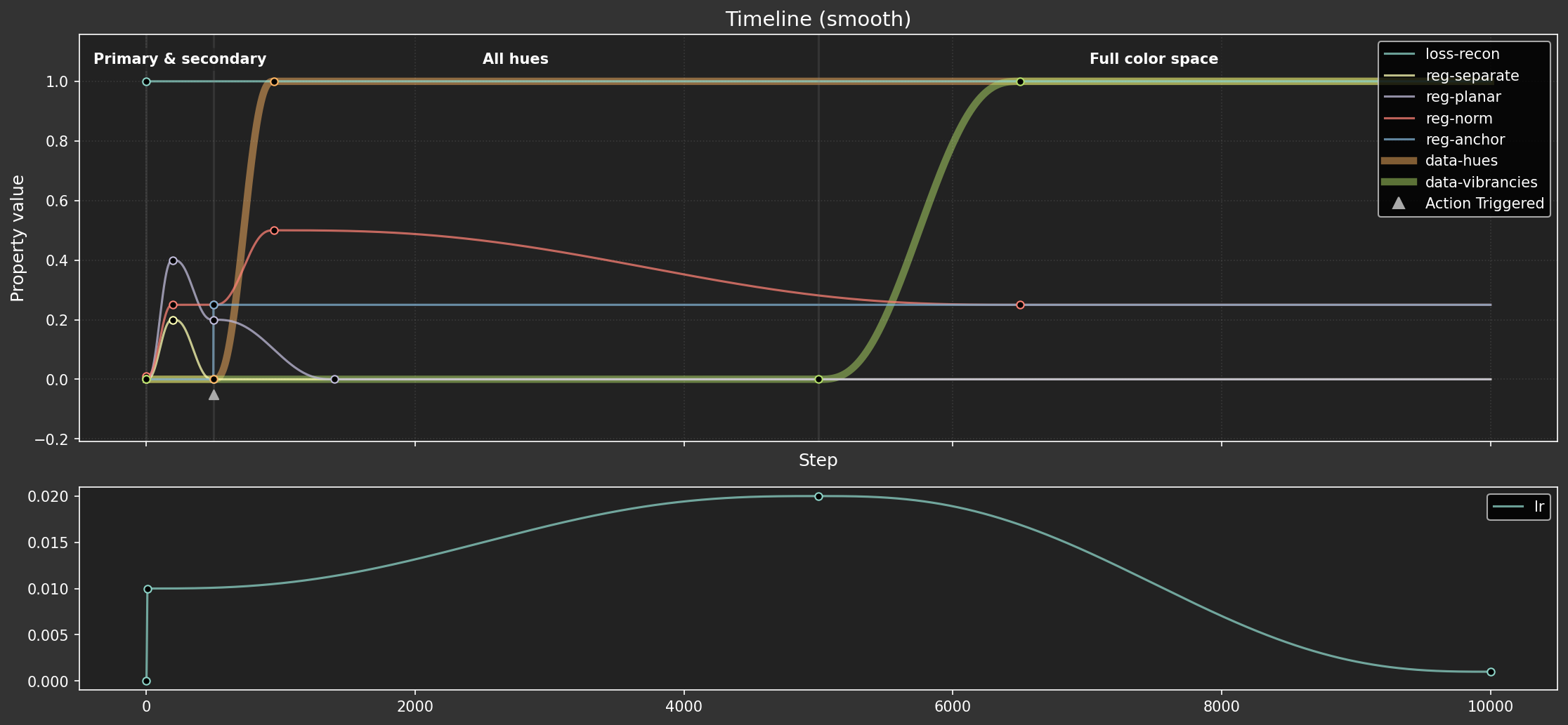
Dopesheets for smooth and stepped curricula
We'll define two dopesheets (timelines):
- The smooth dopesheet uses the eased timing function that was used in the previous experiment.
- The stepped dopesheet uses a step-end timing function.
Apart from the stepped nature of the second, the curricula are almost the same, and both were tuned to give the best performance possible (within reasonable effort limits). To make it fair, the stepped sheet:
- Has more phases, to allow more hyperparameter values
- Uses a learning rate warmup at the start of each phase, since this is already a common practice in curriculum learning.
import re

from IPython.display import display, HTML
from matplotlib import pyplot as plt
from matplotlib.figure import Figure

from mini.temporal.vis import group_properties_by_scale, plot_timeline, realize_timeline, ParamGroup
from mini.temporal.dopesheet import Dopesheet
from mini.temporal.timeline import Timeline
from utils.nb import save_fig


line_styles = [
    (re.compile(r'^data-'), {'linewidth': 5, 'zorder': -1, 'alpha': 0.5}),
    # (re.compile(r'-(anchor|norm)$'), {'linewidth': 2, 'linestyle': (0, (8, 1, 1, 1))}),
]


def load_dopesheet(variant: str):
    dopesheet = Dopesheet.from_csv(f'ex-{nbid}-{variant}-dopesheet.csv')
    # display(Markdown(f"""## Parameter schedule ({variant})\n{dopesheet.to_markdown()}"""))

    timeline = Timeline(dopesheet)
    history_df = realize_timeline(timeline)
    keyframes_df = dopesheet.as_df()

    groups = (
        ParamGroup(
            name='',
            params=[p for p in dopesheet.props if p not in {'lr'}],
            height_ratio=2,
        ),
        ParamGroup(
            name='',
            params=[p for p in dopesheet.props if p in {'lr'}],
            height_ratio=1,
        ),
    )
    # groups = group_properties_by_scale(keyframes_df[dopesheet.props])
    fig, ax = plot_timeline(history_df, keyframes_df, groups, title=f'Timeline ({variant})', line_styles=line_styles)
    # Add assertion to satisfy type checker
    assert isinstance(fig, Figure), 'plot_timeline should return a Figure'
    display(
        HTML(
            save_fig(
                fig,
                f'large-assets/ex-{nbid}-color-timeline-{variant}.png',
                alt_text=f'Line chart showing the {variant} hyperparameter schedule over time.',
            )
        )
    )
    return dopesheet


smooth_dopesheet = load_dopesheet('smooth')
stepped_dopesheet = load_dopesheet('stepped')
Parameter schedule (smooth)
| STEP | PHASE | ACTION | lr | loss-recon | reg-separate | reg-planar | reg-norm | reg-anchor | data-hues | data-vibrancies |
|---|---|---|---|---|---|---|---|---|---|---|
| 0 | Primary & secondary | 1e-08 | 1 | 0 | 0 | 0.01 | 0 | 0 | 0 | |
| 10 | 0.01 | |||||||||
| 200 | 0.2 | 0.4 | 0.25 | |||||||
| 300 | ||||||||||
| 499 | 0 | |||||||||
| 500 | All hues | anchor | 0 | 0.2 | 0.25 | 0.25 | 0 | |||
| 950 | 0.5 | 1 | ||||||||
| 1400 | 0 | |||||||||
| 4999 | ||||||||||
| 5000 | Full color space | 0.02 | 0 | |||||||
| 5010 | ||||||||||
| 6500 | 0.25 | 1 | ||||||||
| 7500 | ||||||||||
| 10000 | 0.001 |
I 3332.5 ut.nb:Figure saved: 'large-assets/ex-1.6-color-timeline-smooth.png'
Parameter schedule (stepped)
| STEP | PHASE | ACTION | lr | loss-recon | reg-separate | reg-planar | reg-norm | reg-anchor | data-hues | data-vibrancies |
|---|---|---|---|---|---|---|---|---|---|---|
| 0 | Primary & secondary | 1e-08 | 1 | 0 | 0.2 | 0.01 | 0 | 0 | 0 | |
| 10 | 0.01 | |||||||||
| 90 | 0.01 | |||||||||
| 100 | Primary & secondary | 1e-08 | 0.15 | 0.3 | 0.25 | |||||
| 110 | 0.01 | |||||||||
| 290 | 0.01 | |||||||||
| 300 | Primary & secondary | 1e-08 | 0 | 0.2 | ||||||
| 310 | 0.01 | |||||||||
| 490 | 0.01 | |||||||||
| 500 | All hues | anchor | 1e-08 | 0.1 | 0.25 | 0.5 | 0 | |||
| 510 | 0.01 | |||||||||
| 990 | 0.0125 | |||||||||
| 1000 | All hues | 1e-08 | 0 | 0.4 | 1 | |||||
| 1010 | 0.0125 | |||||||||
| 4990 | 0.02 | |||||||||
| 5000 | Full color space | 1e-08 | 0.25 | 0.5 | ||||||
| 5010 | 0.02 | |||||||||
| 6490 | 0.016 | |||||||||
| 6500 | Full color space | 1e-08 | 1 | |||||||
| 6510 | 0.016 | |||||||||
| 10000 | 0.001 |
I 3333.4 ut.nb:Figure saved: 'large-assets/ex-1.6-color-timeline-stepped.png'
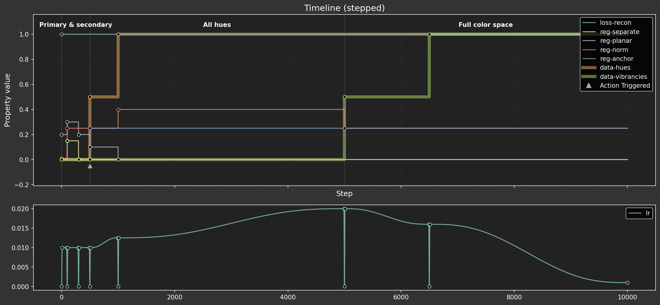
These schedules seem pretty well matched for a fair comparison. The core hyperparameter targets are hit at similar times, with the main difference being, well, the smoothness. This should give us a good basis for seeing what impact the transition style has.
Loss functions and regularizers
Like Ex 1.5, we use mean squared error for the main reconstruction loss (loss-recon), and regularizers that encourage embeddings of unit length, and for primary colors to be on the plane of the first two dimensions.
Unlike Ex 1.5, most of the criteria and regularizers now return per-sample loss, which allows new samples to be given lower weight (see data loaders below).
from torch import linalg as LA

from ex_color.data.color_cube import ColorCube
from ex_color.data.cyclic import arange_cyclic


def objective(fn):
    """Adapt loss function to look like a regularizer"""

    def wrapper(data: Tensor, res: InferenceResult) -> Tensor:
        loss = fn(data, res.outputs)
        # Reduce element-wise loss to per-sample loss by averaging over feature dimensions
        if loss.ndim > 1:
            # Calculate mean over all dimensions except the first (batch) dimension
            reduce_dims = tuple(range(1, loss.ndim))
            loss = torch.mean(loss, dim=reduce_dims)
        return loss

    return wrapper


def unitarity(data: Tensor, res: InferenceResult) -> Tensor:
    """Regularize latents to have unit norm (vectors of length 1)"""
    norms = LA.vector_norm(res.latents, dim=-1)
    # Return per-sample loss, shape [B]
    return (norms - 1.0) ** 2


def planarity(data: Tensor, res: InferenceResult) -> Tensor:
    """Regularize latents to be planar in the first two channels (so zero in other channels)"""
    if res.latents.shape[1] <= 2:
        # No dimensions beyond the first two, return zero loss per sample
        return torch.zeros(res.latents.shape[0], device=res.latents.device)
    # Sum squares across the extra dimensions for each sample, shape [B]
    return torch.sum(res.latents[:, 2:] ** 2, dim=-1)


class Separate(LossCriterion):
    def __init__(self, channels: tuple[int, ...] = (0, 1)):
        self.channels = channels

    def __call__(self, data: Tensor, res: InferenceResult) -> Tensor:
        """
        Regularize latents to be separated from each other in first two channels.

        Returns:
            loss: Per-sample loss, shape [B].
        """
        # Get pairwise differences in the first two dimensions
        points = res.latents[:, self.channels]  # [B, C]
        diffs = points.unsqueeze(1) - points.unsqueeze(0)  # [B, B, C]

        # Calculate squared distances
        sq_dists = torch.sum(diffs**2, dim=-1)  # [B, B]

        # Remove self-distances (diagonal)
        mask = 1.0 - torch.eye(sq_dists.shape[0], device=sq_dists.device)
        masked_sq_dists = sq_dists * mask

        # Encourage separation by minimizing inverse distances (stronger repulsion between close points)
        epsilon = 1e-6  # Prevent division by zero
        return torch.mean(1.0 / (masked_sq_dists + epsilon))


class Anchor(SpecialLossCriterion):
    """Regularize latents to be close to their position in the reference phase"""

    ref_data: Tensor
    _ref_latents: Tensor | None = None

    def __init__(self, ref_data: Tensor):
        self.ref_data = ref_data
        self._ref_latents = None
        log.info(f'Anchor initialized with reference data shape: {ref_data.shape}')

    def forward(self, model: ColorMLP, data: Tensor) -> InferenceResult | None:
        """Run the *stored reference data* through the *current* model."""
        if self._ref_latents is None:
            # Signal to the training loop that we haven't captured latents yet
            return None

        # Note: The 'data' argument passed by the training loop for SpecialLossCriterion
        # is the *current training batch*, which we IGNORE here.
        # We only care about running our stored _ref_data through the model.
        device = next(model.parameters()).device
        ref_data = self.ref_data.to(device)

        outputs, latents = model(ref_data)
        return InferenceResult(outputs, latents)

    def __call__(self, data: Tensor, special: InferenceResult) -> Tensor:
        """
        Calculates loss between current model's latents (for ref_data) and the stored reference latents.

        Returns:
            loss: Mean loss, shape [] (scalar).
        """
        if self._ref_latents is None:
            # This means on_anchor hasn't been called yet, so the anchor loss is zero.
            raise RuntimeError('Anchor.__call__ invoked before reference latents captured. Returning zero loss.')
        ref_latents = self._ref_latents.to(special.latents.device)
        return torch.mean((special.latents - ref_latents) ** 2)

    def on_anchor(self, event: Event):
        # Called when the 'anchor' event is triggered
        log.info(f'Capturing anchor latents via Anchor.on_anchor at step {event.step}')

        device = next(event.model.parameters()).device
        ref_data = self.ref_data.to(device)

        with torch.no_grad():
            _, latents = event.model(ref_data)
        self._ref_latents = latents.detach().cpu()
        log.info(f'Anchor state captured internally. Ref data: {ref_data.shape}, Ref latents: {latents.shape}')
Data loading, sampling, and event handling
Here we set up:
- Datasets: Define the datasets used (primary/secondary colors, full color grid).
- Sampler: Use
DynamicWeightedRandomBatchSamplerfor the full dataset. Its weights are updated by theupdate_sampler_weightscallback, which responds to thedata-fractionparameter from the dopesheet. This smoothly shifts the sampling focus from highly vibrant colors early on to the full range of colors later. - Recorders:
ModelRecorderandMetricsRecorderare event handlers that save the model state and loss values at each step. - Event bindings: Connect event handlers to specific events (e.g.,
plottertophase-end,reg_anchor.on_anchortoaction:anchor, recorders topre-stepandstep-metrics). - Training execution: Finally, call
train_color_modelwith the model, datasets, dopesheet, loss criteria, and configured event handlers.
import numpy as np
import torch.nn as nn


class ModelRecorder(EventHandler):
    """Event handler to record model parameters."""

    history: list[tuple[int, dict[str, Tensor]]]
    """A list of tuples (step, state_dict) where state_dict is a copy of the model's state dict."""

    def __init__(self):
        self.history = []

    def __call__(self, event: Event):
        # Get a *copy* of the state dict and move it to the CPU
        # so we don't hold onto GPU memory or track gradients unnecessarily.
        model_state = {k: v.cpu().clone() for k, v in event.model.state_dict().items()}
        self.history.append((event.step, model_state))
        log.debug(f'Recorded model state at step {event.step}')


class MetricsRecorder(EventHandler):
    """Event handler to record training metrics."""

    history: list[tuple[int, float, dict[str, float]]]
    """A list of tuples (step, total_loss, losses_dict)."""

    def __init__(self):
        self.history = []

    def __call__(self, event: StepMetricsEvent):
        # Ensure we are handling the correct event type
        if not isinstance(event, StepMetricsEvent):
            log.warning(f'MetricsRecorder received unexpected event type: {type(event)}')
            return

        self.history.append((event.step, event.total_loss, event.losses.copy()))
        log.debug(f'Recorded metrics at step {event.step}: loss={event.total_loss:.4f}')
Weighted samples
We add a data collation function, so that as the schedule progresses, new samples are given lower weight. This prevents the optimizer from being too shocked by the previously out-of-distribution data. Without this, we found it wasn't possible to get a smooth loss metric even with the gradual introduction of less-vibrant colors.
from functools import partial
from typing import Callable
import torch
from torch.utils.data import DataLoader, TensorDataset
from torch.utils.data.dataloader import default_collate

# TODO: remove forced reload
if True:
    import importlib
    import ex_color.data.cube_sampler

    importlib.reload(ex_color.data.cube_sampler)

from ex_color.data.cube_sampler import DynamicWeightedRandomBatchSampler, Weights, vibrancy, primary_secondary_focus
from ex_color.data.filters import levels


def ones_collate_fn(batch):
    """Collate data and add a tensor of ones for weights."""
    # TensorDataset yields tuples like ((data_point_tensor,), index_scalar_tensor)
    data_tuple_list = [item[0] for item in batch]  # List of (data_tensor,) tuples
    # indices = [item[1].item() for item in batch] # We don't need indices here

    collated_data = default_collate(data_tuple_list)
    # Create weights tensor of ones, matching batch size and on the same device
    batch_weights = torch.ones(collated_data.shape[0], dtype=torch.float32)
    return collated_data, batch_weights


def weighted_collate_fn(batch, *, get: Callable[[], np.ndarray]):
    """
    Custom collate function that retrieves weights for the sampled indices.

    Args:
        batch: A list of ((data_tensor,), index_tensor) tuples from TensorDataset.
               Note: TensorDataset wraps single tensors in a tuple.
        get: A callable that returns the current full sampler weights array.

    Returns:
        A tuple: (collated_data_tensor, collated_weights_tensor)
    """
    # Separate data and indices
    # TensorDataset yields tuples like ((data_point_tensor,), index_scalar_tensor)
    data_tuple_list = [item[0] for item in batch]  # List of (data_tensor,) tuples
    indices = [item[1].item() for item in batch]  # List of integer indices

    # Collate the data points using the default collate function
    # default_collate handles the list of (data_tensor,) tuples correctly
    collated_data = default_collate(data_tuple_list)

    # Look up weights for the indices in this batch
    # Ensure weights are float32 for potential multiplication with loss
    sampler_weights = get()
    batch_weights = torch.tensor(sampler_weights[indices], dtype=torch.float32)

    # Normalize weights within the batch? Or use raw weights?
    # Let's use raw weights for now, as they reflect the sampling probability.
    # If weights sum to zero (unlikely but possible if all sampled points have zero weight),
    # avoid division by zero.
    weight_sum = batch_weights.sum()
    if weight_sum > 1e-6:
        batch_weights /= weight_sum
    else:
        # Assign uniform weight if sum is zero
        batch_weights = torch.ones_like(batch_weights) / len(batch_weights)

    return collated_data, batch_weights


primary_cube = ColorCube.from_hsv(h=arange_cyclic(step_size=1 / 6), s=np.ones(1), v=np.ones(1))
primary_tensor = torch.tensor(primary_cube.rgb_grid.reshape(-1, 3), dtype=torch.float32)
primary_dataset = TensorDataset(primary_tensor)
primary_loader = DataLoader(
    primary_dataset,
    batch_size=len(primary_tensor),
    collate_fn=ones_collate_fn,
)

full_cube = ColorCube.from_hsv(
    h=arange_cyclic(step_size=10 / 360),
    s=np.linspace(0, 1, 10),
    v=np.linspace(0, 1, 10),
)
full_tensor = torch.tensor(full_cube.rgb_grid.reshape(-1, 3), dtype=torch.float32)
full_dataset = TensorDataset(full_tensor, torch.arange(len(full_tensor)))
full_sampler = DynamicWeightedRandomBatchSampler(
    bias=full_cube.bias.flatten(),
    batch_size=32,
    steps_per_epoch=100,
)
primary_secondary_weights = primary_secondary_focus(full_cube).flatten()
vibrancy_weights = vibrancy(full_cube).flatten()
full_loader = DataLoader(
    full_dataset,
    batch_sampler=full_sampler,
    collate_fn=partial(weighted_collate_fn, get=lambda: full_sampler.weights),
)

rgb_cube = ColorCube.from_rgb(
    r=np.linspace(0, 1, 8),
    g=np.linspace(0, 1, 8),
    b=np.linspace(0, 1, 8),
)
rgb_tensor = torch.tensor(rgb_cube.rgb_grid.reshape(-1, 3), dtype=torch.float32)


def scale_weights(weights: Weights, frac: float) -> Weights:
    # When the fraction is near zero, in_low is almost 1 — which means "scale everything down to 0 except for 1"
    # When the fraction is 0.5, in_low and out_low are both 0, so the weights are unchanged
    # When the fraction is 1, in_low is 0 and out_low is 1, so the weights are all scaled to 1
    in_low = np.interp(frac, [0, 0.5], [0.99, 0])
    out_low = np.interp(frac, [0.5, 1], [0, 1])
    return levels(weights, in_low=in_low, out_low=out_low)


def update_sampler_weights(event: Event):
    """Event handler to update sampler weights based on the current hyperparameters."""
    hue_frac = event.timeline_state.props['data-hues']
    vibrancy_frac = event.timeline_state.props['data-vibrancies']

    scaled_vibrancy_weights = scale_weights(vibrancy_weights, vibrancy_frac)
    scaled_primary_secondary_weights = scale_weights(primary_secondary_weights, hue_frac)
    full_sampler.weights = scaled_vibrancy_weights * scaled_primary_secondary_weights


async def train(dopesheet: Dopesheet, variant: str):
    """Train the model with the given dopesheet and variant."""
    log.info(f'Training with {variant} dopesheet.')
    recorder = ModelRecorder()
    metrics_recorder = MetricsRecorder()

    seed = 0
    set_deterministic_mode(seed)
    full_sampler.seed = seed

    # Phase -> (train loader, validation tensor)
    datasets: dict[str, tuple[DataLoader, Tensor]] = {
        'Primary & secondary': (primary_loader, primary_tensor),
        'All hues': (full_loader, rgb_tensor),
        'Full color space': (full_loader, rgb_tensor),
    }

    model = ColorMLP(normalize_bottleneck=False)
    total_params = sum(p.numel() for p in model.parameters() if p.requires_grad)
    log.info(f'Model initialized with {total_params:,} trainable parameters.')

    event_handlers = EventHandlers()
    event_handlers.pre_step.add_handler('pre-step', recorder)
    event_handlers.pre_step.add_handler('pre-step', update_sampler_weights)
    event_handlers.step_metrics.add_handler('step-metrics', metrics_recorder)

    plotter = PhasePlotter(dim_pairs=[(0, 1), (0, 2), (0, 3)], variant=variant)
    event_handlers.phase_end.add_handler('phase-end', plotter)

    reg_anchor = Anchor(ref_data=primary_tensor)
    event_handlers.action.add_handler('action:anchor', reg_anchor.on_anchor)

    await train_color_model(
        model,
        datasets,
        dopesheet,
        loss_criteria={
            'loss-recon': objective(nn.MSELoss(reduction='none')),  # No reduction; allows per-sample loss weights
            'reg-separate': Separate((0, 1)),
            'reg-planar': planarity,
            'reg-norm': unitarity,
            'reg-anchor': reg_anchor,
        },
        event_handlers=event_handlers,
    )

    return recorder, metrics_recorder
smooth_recorder, smooth_metrics = await train(smooth_dopesheet, 'smooth')
I 3345.2 no.1.6:Training with smooth dopesheet.
I 3345.2 no.1.6:Global random seed set to 0
I 3345.2 no.1.6:PyTorch set to deterministic mode
I 3345.2 no.1.6:Model initialized with 263 trainable parameters.
I 3345.2 no.1.6:Anchor initialized with reference data shape: torch.Size([6, 3])
I 3346.3 no.1.6:Plotting end of phase: Primary & secondary at step 499 using provided results.
I 3346.5 ut.nb:Figure saved: 'large-assets/ex-1.6-color-phase-history-smooth.png'
I 3346.5 no.1.6:Capturing anchor latents via Anchor.on_anchor at step 500
I 3346.5 no.1.6:Anchor state captured internally. Ref data: torch.Size([6, 3]), Ref latents: torch.Size([6, 4])
I 3356.1 no.1.6:Plotting end of phase: All hues at step 4999 using provided results.
I 3356.4 ut.nb:Figure saved: 'large-assets/ex-1.6-color-phase-history-smooth.png'
I 3370.2 no.1.6:Plotting end of phase: Full color space at step 10000 using provided results.
I 3371.6 ut.nb:Figure saved: 'large-assets/ex-1.6-color-phase-history-smooth.png'
I 3371.6 no.1.6:Training finished!
stepped_recorder, stepped_metrics = await train(stepped_dopesheet, 'stepped')
I 3385.8 no.1.6:Training with stepped dopesheet.
I 3385.8 no.1.6:Global random seed set to 0
I 3385.8 no.1.6:PyTorch set to deterministic mode
I 3385.8 no.1.6:Model initialized with 263 trainable parameters.
I 3385.8 no.1.6:Anchor initialized with reference data shape: torch.Size([6, 3])
I 3386.1 no.1.6:Plotting end of phase: Primary & secondary at step 99 using provided results.
I 3386.2 ut.nb:Figure saved: 'large-assets/ex-1.6-color-phase-history-stepped.png'
I 3386.7 no.1.6:Plotting end of phase: Primary & secondary at step 299 using provided results.
I 3387.0 ut.nb:Figure saved: 'large-assets/ex-1.6-color-phase-history-stepped.png'
I 3387.3 no.1.6:Plotting end of phase: Primary & secondary at step 499 using provided results.
I 3387.7 ut.nb:Figure saved: 'large-assets/ex-1.6-color-phase-history-stepped.png'
I 3387.8 no.1.6:Capturing anchor latents via Anchor.on_anchor at step 500
I 3387.8 no.1.6:Anchor state captured internally. Ref data: torch.Size([6, 3]), Ref latents: torch.Size([6, 4])
I 3389.1 no.1.6:Plotting end of phase: All hues at step 999 using provided results.
I 3389.7 ut.nb:Figure saved: 'large-assets/ex-1.6-color-phase-history-stepped.png'
I 3397.9 no.1.6:Plotting end of phase: All hues at step 4999 using provided results.
I 3398.7 ut.nb:Figure saved: 'large-assets/ex-1.6-color-phase-history-stepped.png'
I 3401.9 no.1.6:Plotting end of phase: Full color space at step 6499 using provided results.
I 3402.9 ut.nb:Figure saved: 'large-assets/ex-1.6-color-phase-history-stepped.png'
I 3410.9 no.1.6:Plotting end of phase: Full color space at step 10000 using provided results.
I 3412.2 ut.nb:Figure saved: 'large-assets/ex-1.6-color-phase-history-stepped.png'
I 3412.2 no.1.6:Training finished!
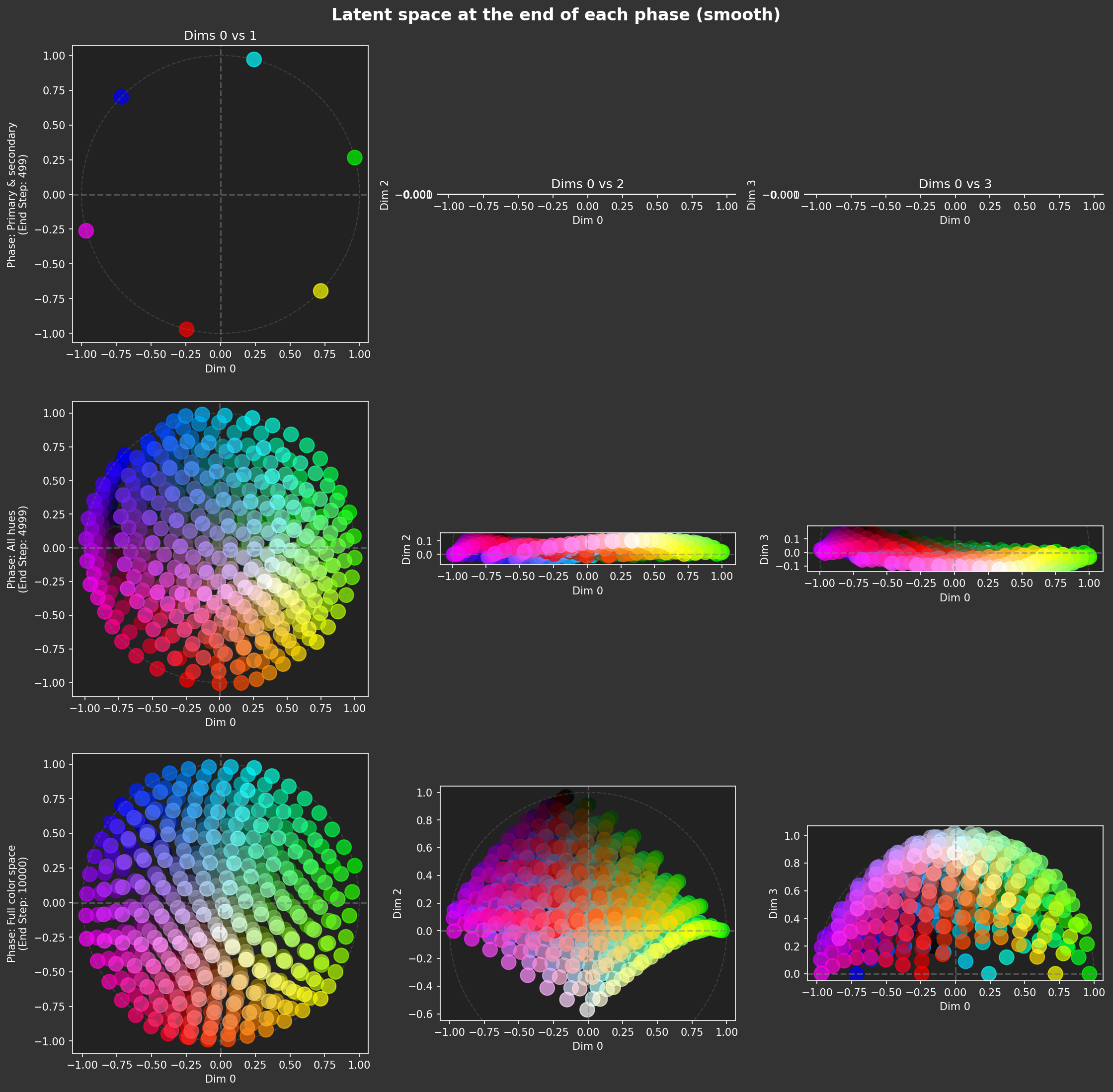
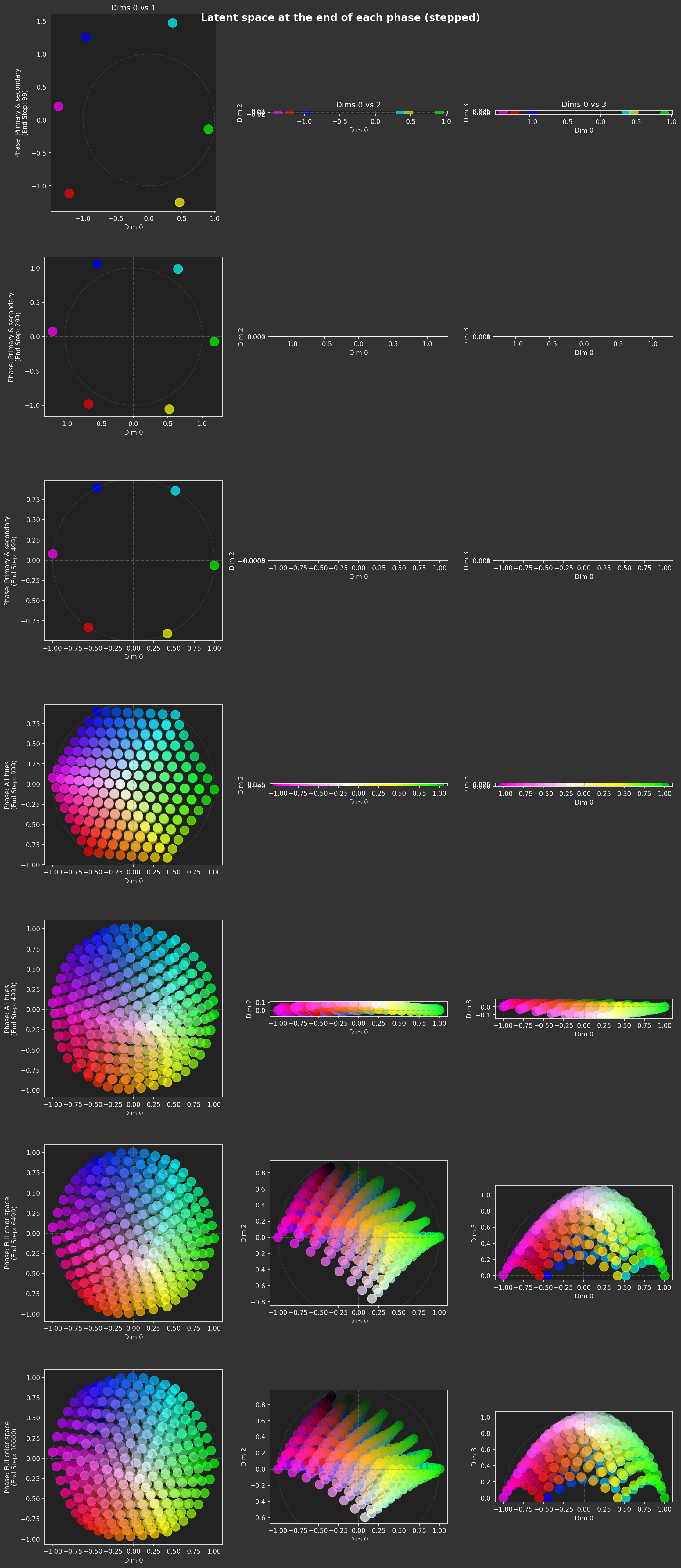
Both models trained fairly well! There are some differences, but they look like they have similar characteristics. Surprisingly, the smooth variant seemed to have a noisier (i.e. worse) latent space at the end of the All hues phase.
Latent space evolution analysis
Let's visualize how the latent spaces evolved over time. Like Ex 1.5, we'll use the ModelRecorder's history to load the model state at each recorded step and evaluate the latent positions for a fixed set of input colors (the full RGB grid). This gives us a sequence of latent space snapshots.
import numpy as np


async def eval_latent_history(
    recorder: ModelRecorder,
    rgb_tensor: Tensor,
):
    """Evaluate the latent space for each step in the recorder's history."""
    # Create a new model instance
    from utils.progress import co_op, Progress

    model = ColorMLP(normalize_bottleneck=False)

    latent_history: list[tuple[int, np.ndarray]] = []
    # Iterate over the recorded history
    async for step, state_dict in co_op(Progress(recorder.history, description='Evaluating latents')):
        # Load the model state dict
        model.load_state_dict(state_dict)
        model.eval()
        with torch.no_grad():
            # Get the latents for the RGB tensor
            _, latents = model(rgb_tensor.to(next(model.parameters()).device))
            latents = latents.cpu().numpy()
            latent_history.append((step, latents))
    return latent_history


smooth_latents = await eval_latent_history(smooth_recorder, rgb_tensor)
stepped_latents = await eval_latent_history(stepped_recorder, rgb_tensor)
Animation of latent space
This final visualization combines multiple views into a single animation:
- Latent space: Shows the 2D projection (Dims 0 vs 1) of the latent embeddings for the full RGB color grid, colored by their true RGB values. We can see the color wheel forming.
- Hyperparameters: Replots the parameter schedule from the dopesheet, with a vertical line indicating the current step in the animation.
- Training metrics: Plots the total loss and the contribution of each individual loss/regularization term (on a log scale), again with a vertical line for the current step.
(Note: A variable stride is used for sampling frames to focus on periods of rapid change.)
The smooth training run is shown on the left, and the stepped run on the right.
import matplotlib.pyplot as plt
import matplotlib.animation as animation
import imageio_ffmpeg
from matplotlib import rcParams
import pandas as pd
from matplotlib.gridspec import GridSpec

from mini.temporal.dopesheet import RESERVED_COLS
from utils.progress import SyncProgress

# TODO: remove forced reload
import importlib
import mini.temporal.vis

importlib.reload(mini.temporal.vis)
from mini.temporal.vis import group_properties_by_scale, plot_timeline

rcParams['animation.ffmpeg_path'] = imageio_ffmpeg.get_ffmpeg_exe()


def animate_latent_evolution_with_metrics(
    # Smooth variant data
    smooth_latent_history: list[tuple[int, np.ndarray]],
    smooth_metrics_history: list[tuple[int, float, dict[str, float]]],
    smooth_param_history_df: pd.DataFrame,
    smooth_param_keyframes_df: pd.DataFrame,
    # Stepped variant data
    stepped_latent_history: list[tuple[int, np.ndarray]],
    stepped_metrics_history: list[tuple[int, float, dict[str, float]]],
    stepped_param_history_df: pd.DataFrame,
    stepped_param_keyframes_df: pd.DataFrame,
    # Common data and settings
    colors: np.ndarray,
    dim_pair: tuple[int, int] = (0, 1),
    interval=1 / 30,
):
    """Create a side-by-side animation of latent space evolution, hyperparameters, and metrics."""
    plt.style.use('dark_background')
    # Aim for 16:9 aspect ratio, give latent plots more height
    fig = plt.figure(figsize=(16, 9))
    # Use the height ratios from your latest version
    gs = GridSpec(3, 2, height_ratios=[5, 1, 1], width_ratios=[1, 1], hspace=0, wspace=0.02)

    # --- Create Axes ---
    # Latent plots (Top row) - No sharing needed initially
    ax_latent_s = fig.add_subplot(gs[0, 0])
    ax_latent_t = fig.add_subplot(gs[0, 1])

    # Parameter plots (Middle row) - Share x-axis with metrics plot BELOW
    ax_params_s = fig.add_subplot(gs[1, 0])
    ax_params_t = fig.add_subplot(gs[1, 1])

    # Metrics plots (Bottom row) - Share x-axis with parameter plot ABOVE
    ax_metrics_s = fig.add_subplot(gs[2, 0], sharex=ax_params_s)
    ax_metrics_t = fig.add_subplot(gs[2, 1], sharex=ax_params_t)

    fig.patch.set_facecolor('#333')
    all_axes = [ax_latent_s, ax_params_s, ax_metrics_s, ax_latent_t, ax_params_t, ax_metrics_t]
    for ax in all_axes:
        ax.patch.set_facecolor('#222')

    latent_lim = 1.1

    # --- Setup Smooth Plots (Left Column) ---
    step_s, current_latents_s = smooth_latent_history[0]
    ax_latent_s.set_xlim(-latent_lim, latent_lim)
    ax_latent_s.set_ylim(-latent_lim, latent_lim)
    ax_latent_s.set_aspect('equal', adjustable='datalim')
    # ax_latent_s.set_xlabel(f'Dim {dim_pair[0]}') # Set X label for latent plot
    ax_latent_s.tick_params(axis='x', labelleft=False)  # Hide x labels
    plt.setp(ax_latent_s.get_xticklabels(), visible=False)
    # ax_latent_s.set_ylabel(f'Dim {dim_pair[1]}')
    ax_latent_s.set_ylabel('Latent space')
    ax_latent_s.axhline(y=0, color='gray', linestyle='--', alpha=0.5)
    ax_latent_s.axvline(x=0, color='gray', linestyle='--', alpha=0.5)
    ax_latent_s.add_patch(Circle((0, 0), 1, fill=False, linestyle='--', color='gray', alpha=0.3))
    scatter_s = ax_latent_s.scatter(
        current_latents_s[:, dim_pair[0]], current_latents_s[:, dim_pair[1]], c=colors, s=150, alpha=0.7
    )
    title_latent_s = ax_latent_s.set_title('placeholder')  # Title set in update()
    # No need to hide x-ticks here anymore

    param_props_s = smooth_param_keyframes_df.columns.difference(list(RESERVED_COLS)).tolist()
    param_groups_s = group_properties_by_scale(smooth_param_keyframes_df[param_props_s])
    # Pass show_legend=False, show_phase_labels=False as you did
    plot_timeline(
        smooth_param_history_df,
        smooth_param_keyframes_df,
        [param_groups_s[0]],
        ax=ax_params_s,
        show_legend=False,
        show_phase_labels=False,
        line_styles=line_styles,
    )
    param_vline_s = ax_params_s.axvline(step_s, color='white', linestyle='--', lw=1)
    ax_params_s.set_ylabel('Param value', fontsize='x-small')
    ax_params_s.set_xlabel('')  # Remove xlabel, it will be on the plot below
    # Hide x-tick labels because they are shared with the plot below
    plt.setp(ax_params_s.get_xticklabels(), visible=False)

    metrics_steps_s = [h[0] for h in smooth_metrics_history]
    total_losses_s = [h[1] for h in smooth_metrics_history]
    loss_components_s = {
        k: [h[2].get(k, np.nan) for h in smooth_metrics_history] for k in smooth_metrics_history[0][2].keys()
    }
    ax_metrics_s.plot(metrics_steps_s, total_losses_s, label='Total Loss', lw=latent_lim)
    for name, values in loss_components_s.items():
        ax_metrics_s.plot(metrics_steps_s, values, label=name, lw=1, alpha=0.8)
    ax_metrics_s.set_xlabel('Step')  # Set X label for the bottom plot
    ax_metrics_s.set_ylabel('Loss (log)', fontsize='x-small')
    ax_metrics_s.set_yscale('log')
    ax_metrics_s.set_ylim(bottom=1e-6)
    metrics_vline_s = ax_metrics_s.axvline(step_s, color='white', linestyle='--', lw=1)

    # --- Setup Stepped Plots (Right Column) ---
    step_t, current_latents_t = stepped_latent_history[0]
    ax_latent_t.set_xlim(-latent_lim, latent_lim)
    ax_latent_t.set_ylim(-latent_lim, latent_lim)
    ax_latent_t.set_aspect('equal', adjustable='datalim')
    # ax_latent_t.set_xlabel(f'Dim {dim_pair[0]}') # Set X label for latent plot
    ax_latent_t.tick_params(axis='x', labelleft=False)  # Hide x labels
    plt.setp(ax_latent_t.get_xticklabels(), visible=False)
    ax_latent_t.tick_params(axis='y', labelleft=False)  # Hide y labels
    ax_latent_t.axhline(y=0, color='gray', linestyle='--', alpha=0.5)
    ax_latent_t.axvline(x=0, color='gray', linestyle='--', alpha=0.5)
    ax_latent_t.add_patch(Circle((0, 0), 1, fill=False, linestyle='--', color='gray', alpha=0.3))
    scatter_t = ax_latent_t.scatter(
        current_latents_t[:, dim_pair[0]], current_latents_t[:, dim_pair[1]], c=colors, s=150, alpha=0.7
    )
    title_latent_t = ax_latent_t.set_title('placeholder')  # Title set in update()
    # No need to hide x-ticks here anymore

    param_props_t = stepped_param_keyframes_df.columns.difference(list(RESERVED_COLS)).tolist()
    param_groups_t = group_properties_by_scale(stepped_param_keyframes_df[param_props_t])
    # Pass show_legend=False, show_phase_labels=False as you did
    plot_timeline(
        stepped_param_history_df,
        stepped_param_keyframes_df,
        [param_groups_t[0]],
        ax=ax_params_t,
        show_legend=False,
        show_phase_labels=False,
        line_styles=line_styles,
    )
    param_vline_t = ax_params_t.axvline(step_t, color='white', linestyle='--', lw=1)
    ax_params_t.set_ylabel('')  # Y label only on left
    ax_params_t.set_xlabel('')  # Remove xlabel, it will be on the plot below
    # Hide x-tick labels because they are shared with the plot below
    plt.setp(ax_params_t.get_xticklabels(), visible=False)
    ax_params_t.tick_params(axis='y', labelleft=False)  # Hide y labels

    metrics_steps_t = [h[0] for h in stepped_metrics_history]
    total_losses_t = [h[1] for h in stepped_metrics_history]
    loss_components_t = {
        k: [h[2].get(k, np.nan) for h in stepped_metrics_history] for k in stepped_metrics_history[0][2].keys()
    }
    ax_metrics_t.plot(metrics_steps_t, total_losses_t, label='Total Loss', lw=1.5)
    for name, values in loss_components_t.items():
        ax_metrics_t.plot(metrics_steps_t, values, label=name, lw=1, alpha=0.8)
    ax_metrics_t.set_xlabel('Step')  # Set X label for the bottom plot
    ax_metrics_t.set_yscale('log')
    ax_metrics_t.set_ylim(bottom=1e-6)
    ax_metrics_t.tick_params(axis='y', labelleft=False)  # Hide y labels
    metrics_vline_t = ax_metrics_t.axvline(step_t, color='white', linestyle='--', lw=1)

    # --- Set common X limits ---
    # Only set xlim for the timeline plots (params and metrics)
    max_step = max(smooth_param_history_df['STEP'].max(), stepped_param_history_df['STEP'].max())
    for ax in [ax_params_s, ax_metrics_s, ax_params_t, ax_metrics_t]:
        ax.set_xlim(left=0, right=max_step)

    # fig.tight_layout(h_pad=0, w_pad=0.5)  # Adjust padding
    fig.subplots_adjust(
        left=0.05,  # Smaller left margin
        right=0.95,  # Smaller right margin
        bottom=0.08,  # Smaller bottom margin (leave room for x-label)
        top=0.95,  # Smaller top margin (leave room for titles)
        wspace=0.1,  # Adjust space between columns (tweak as needed)
        hspace=0.0,  # Keep vertical space at 0 (set in GridSpec)
    )

    def update(frame: int):
        # ... (update logic remains the same) ...
        # Assume smooth and stepped histories have the same length and aligned steps after sampling
        smooth_step, current_latents_s = smooth_latent_history[frame]
        stepped_step, current_latents_t = stepped_latent_history[frame]
        # Use the smooth step for titles and lines, assuming they are aligned
        current_step = smooth_step

        # Update smooth plots
        scatter_s.set_offsets(current_latents_s[:, dim_pair])
        title_latent_s.set_text(f'Smooth curriculum (step {current_step})')  # Use current_step
        param_vline_s.set_xdata([current_step])
        metrics_vline_s.set_xdata([current_step])

        # Update stepped plots
        scatter_t.set_offsets(current_latents_t[:, dim_pair])
        title_latent_t.set_text(f'Stepped curriculum (step {current_step})')  # Use current_step
        param_vline_t.set_xdata([current_step])
        metrics_vline_t.set_xdata([current_step])

        return (
            scatter_s,
            title_latent_s,
            param_vline_s,
            metrics_vline_s,
            scatter_t,
            title_latent_t,
            param_vline_t,
            metrics_vline_t,
        )

    # Use the length of the (potentially strided) latent_history for frames
    # Assuming both histories have the same length after sampling
    num_frames = len(smooth_latent_history)
    ani = animation.FuncAnimation(fig, update, frames=num_frames, interval=interval * 1000, blit=True)
    return fig, ani


# --- Variable Stride Logic ---
def get_stride(step: int):
    import math

    a = 7.9236
    b = 0.0005
    # Ensure stride is at least 1
    return max(1.0, a * math.log(b * step + 1) + 1)


# Apply stride logic based on smooth history (assuming stepped is similar)
sampled_indices = [0]
last_sampled_index = 0
# Use smooth_latents for stride calculation
while True:
    current_step = smooth_latents[round(last_sampled_index)][0]
    stride = get_stride(current_step)
    next_index = last_sampled_index + stride
    # Ensure indices stay within bounds for *both* histories
    if round(next_index) >= len(smooth_latents) or round(next_index) >= len(stepped_latents):
        break
    sampled_indices.append(round(next_index))
    last_sampled_index = next_index

# Ensure the last frame is included if missed
if sampled_indices[-1] < len(smooth_latents) - 1:
    sampled_indices.append(len(smooth_latents) - 1)

# sampled_indices = sampled_indices[:200]  # Limit the number of samples during development

# Sample both latent histories using the same indices
sampled_smooth_latents = [smooth_latents[i] for i in sampled_indices]
sampled_stepped_latents = [stepped_latents[i] for i in sampled_indices]

# --- End Variable Stride Logic ---

# Filter metrics history to align with the *new* sampled latent history steps
# Use steps from the sampled smooth history (assuming alignment)
sampled_steps_set = {step for step, _ in sampled_smooth_latents}
filtered_smooth_metrics = [h for h in smooth_metrics.history if h[0] in sampled_steps_set]
filtered_stepped_metrics = [h for h in stepped_metrics.history if h[0] in sampled_steps_set]

# Realize timelines for both dopesheets
smooth_timeline = Timeline(smooth_dopesheet)
smooth_history_df = realize_timeline(smooth_timeline)
smooth_keyframes_df = smooth_dopesheet.as_df()

stepped_timeline = Timeline(stepped_dopesheet)
stepped_history_df = realize_timeline(stepped_timeline)
stepped_keyframes_df = stepped_dopesheet.as_df()


# --- Call the updated animation function ---
fig, ani = animate_latent_evolution_with_metrics(
    # Smooth
    smooth_latent_history=sampled_smooth_latents,
    smooth_metrics_history=filtered_smooth_metrics,
    smooth_param_history_df=smooth_history_df,
    smooth_param_keyframes_df=smooth_keyframes_df,
    # Stepped
    stepped_latent_history=sampled_stepped_latents,
    stepped_metrics_history=filtered_stepped_metrics,
    stepped_param_history_df=stepped_history_df,
    stepped_param_keyframes_df=stepped_keyframes_df,
    # Common
    colors=rgb_tensor.cpu().numpy(),
    dim_pair=(0, 1),
)

# --- Save the video ---
video_file = f'large-assets/ex-{nbid}-latent-evolution-comparison.mp4'  # Updated filename
num_frames_to_render = len(sampled_smooth_latents)  # Base on sampled length
with SyncProgress(total=num_frames_to_render, description='Rendering comparison video') as pbar:
    ani.save(
        video_file,
        fps=30,
        extra_args=['-vcodec', 'libx264'],
        progress_callback=lambda i, n: pbar.update(total=n, count=i),
    )
plt.close(fig)

# --- Display the video ---
import secrets
from IPython.display import display, HTML

cache_buster = secrets.token_urlsafe()

display(
    HTML(
        f"""
        <video width="960" height="540" controls loop>
            <source src="{video_file}?v={cache_buster}" type="video/mp4">
            Your browser does not support the video tag.
        </video>
        """
    )
)
W 3444.3 ma.ax._b:Ignoring fixed x limits to fulfill fixed data aspect with adjustable data limits.
W 3444.3 ma.ax._b:Ignoring fixed x limits to fulfill fixed data aspect with adjustable data limits.
Observations
Qualitatively, we observe that:
- The Smooth variant seems noisier overall: it's more jittery in general, and becomes more misshapen during the All hues phase. This might be due to the specific values of the hyperparameters, e.g. maybe the normalization loss was too high.
- The Stepped variant does indeed show loss spikes at the start of each phase, while the Smooth varint does not — as predicted! However, the spikes don't seem to cause any problem; perhaps they were fully mitigated by the LR warmup.
- Even though the data are introduced to each variant differently (in chunks to the Stepped variant, and gradually to the Smooth variant), the effect is almost identical. This is particularly apparent at the start of the Full color space phase: the Stepped variant bulges suddenly at the start of the phase, while the Smooth variant bulges a little later and somewhat less violently — but both end up in almost the exact same shape.
Perhaps the dynamics and final latent space could be improved for the Smooth curriculum by reducing the learning rate at times when the parameters are changing a lot — but since per-phase LR schedules are already common in curriculum learning, using them in addition to smooth parameter changes may not have much benefit. On the other hand, we note that the smooth curriculum was easier to specify than the stepped one, purely because it had fewer phases and fewer keyframes.
Conclusion
Our hypothesis seems to have been wrong: smooth parameter changes don't appear to improve training dynamics compared to a traditional curriculum.