Experiment 2.9: Delete only red with extra nonlinearity
In Ex 2.8, we attempted to delete only red without also deleting cyan. We expected that simply adding an "anti anchor" regularization term would work by keeping all colors away from the direction opposing red. It did that, but the ablation removed far more than red. We think the combination of regularization terms may have added too many constraints for the model architecture to resolve.
Hypothesis
If we add more dimensions to the bottleneck and more layers to the encoder and decoder, the model will be able to warp latent space enough to satisfy the constraints of the regularizers, and we will be able to delete red without also deleting other colors.
When we look at latent space, I imagine we might see a more pronounced protrusion of reds into the hemi-hypersphere of the first dimension — something like a flat base with a blob rising from it.
from __future__ import annotations

nbid = '2.9'  # ID for tagging assets
nbname = 'Ablate red (only), 5D'
experiment_name = f'Ex {nbid}: {nbname}'
project = 'ex-preppy'
# Basic setup: Logging, Experiment (Modal)
import logging

import modal

from infra.requirements import freeze, project_packages
from mini.experiment import Experiment
from utils.logging import SimpleLoggingConfig

logging_config = (
    SimpleLoggingConfig()
    .info('notebook', 'utils', 'mini', 'ex_color')
    .error('matplotlib.axes')  # Silence warnings about set_aspect
)
logging_config.apply()

# This is the logger for this notebook
log = logging.getLogger(f'notebook.{nbid}')

run = Experiment(experiment_name, project=project)
run.image = modal.Image.debian_slim().pip_install(*freeze(all=True)).add_local_python_source(*project_packages())
run.before_each(logging_config.apply)
None  # prevent auto-display of this cell
Regularizers
Like Ex 2.8:
- Anchor: pins
redto $(1,0,0,0,0)$ (but note it's now 5D) - Anti-anchor: repels everything from $(-1,0,0,0,0)$ (now 5D)
- Separate: angular repulsion to reduce global clumping (applied within each batch)
- Unitarity: pulls all embeddings to the surface of the unit hypersphere, i.e. it makes the embedding vectors have unit length.
But unlike 2.8:
- AxisAlignedSubspace: the planarity constraint has been brought back, but this time it is inverted: it targets desaturated colors, and keeps them out of the first two dimensions.
import torch

from mini.temporal.dopesheet import Dopesheet
from ex_color.loss import AngularAnchor, AntiAnchor, Separate, Unitarity, AxisAlignedSubspace, RegularizerConfig

from ex_color.training import TrainingModule

K = 5  # bottleneck dimensionality
RED = (1, 0, 0, 0, 0)
ANTI_RED = tuple(-c for c in RED)
assert len(RED) == len(ANTI_RED) == K

ALL_REGULARIZERS = [
    RegularizerConfig(
        name='reg-unit',
        compute_loss_term=Unitarity(),
        label_affinities=None,
        layer_affinities=['encoder'],
    ),
    RegularizerConfig(
        name='reg-anchor',
        compute_loss_term=AngularAnchor(torch.tensor(RED, dtype=torch.float32)),
        label_affinities={'red': 1.0},
        layer_affinities=['bottleneck'],
    ),
    RegularizerConfig(
        name='reg-separate',
        compute_loss_term=Separate(power=100.0, shift=True),
        label_affinities=None,
        layer_affinities=['bottleneck'],
    ),
    RegularizerConfig(
        name='reg-planar-d',
        compute_loss_term=AxisAlignedSubspace((2, 3, 4)),
        label_affinities={'desaturated': 1.0},
        layer_affinities=['bottleneck'],
    ),
    RegularizerConfig(
        name='reg-anti-anchor',
        compute_loss_term=AntiAnchor(torch.tensor(ANTI_RED, dtype=torch.float32)),
        label_affinities=None,
        layer_affinities=['bottleneck'],
    ),
]
from functools import partial
from torch import Tensor
from torch.utils.data import DataLoader, TensorDataset, WeightedRandomSampler
import numpy as np

from ex_color.data.color_cube import ColorCube
from ex_color.data.cube_sampler import vibrancy
from ex_color.data.cyclic import arange_cyclic
from ex_color.labelling import collate_with_generated_labels


def prep_data() -> tuple[DataLoader, Tensor]:
    """
    Prepare data for training.

    Returns: (train, val)
    """
    hsv_cube = ColorCube.from_hsv(
        h=arange_cyclic(step_size=10 / 360),
        s=np.linspace(0, 1, 10),
        v=np.linspace(0, 1, 10),
    )
    hsv_tensor = torch.tensor(hsv_cube.rgb_grid.reshape(-1, 3), dtype=torch.float32)
    vibrancy_tensor = torch.tensor(vibrancy(hsv_cube).flatten(), dtype=torch.float32)
    hsv_dataset = TensorDataset(hsv_tensor, vibrancy_tensor)

    labeller = partial(
        collate_with_generated_labels,
        soft=False,  # Use binary labels (stochastic) to simulate the labelling of internet text
        red=0.5,
        vibrant=0.5,
        desaturated=0.5,
    )
    # Desaturated and dark colors are over-represented in the cube, so we use a weighted sampler to balance them out
    hsv_loader = DataLoader(
        hsv_dataset,
        batch_size=64,
        num_workers=2,
        sampler=WeightedRandomSampler(
            weights=hsv_cube.bias.flatten().tolist(),
            num_samples=len(hsv_dataset),
            replacement=True,
        ),
        collate_fn=labeller,
    )

    rgb_cube = ColorCube.from_rgb(
        r=np.linspace(0, 1, 8),
        g=np.linspace(0, 1, 8),
        b=np.linspace(0, 1, 8),
    )
    rgb_tensor = torch.tensor(rgb_cube.rgb_grid.reshape(-1, 3), dtype=torch.float32)
    return hsv_loader, rgb_tensor
import wandb
from ex_color.model import CNColorMLP


# @run.thither(env={'WANDB_API_KEY': wandb.Api().api_key})
async def train(
    dopesheet: Dopesheet,
    regularizers: list[RegularizerConfig],
    k_bottleneck: int,
) -> CNColorMLP:
    """Train the model with the given dopesheet and variant."""
    import lightning as L
    from lightning.pytorch.loggers import WandbLogger

    from ex_color.seed import set_deterministic_mode

    from utils.progress.lightning import LightningProgress

    log.info(f'Training with: {[r.name for r in regularizers]}')

    seed = 0
    set_deterministic_mode(seed)

    hsv_loader, _ = prep_data()

    model = CNColorMLP(k_bottleneck, n_nonlinear=2)
    total_params = sum(p.numel() for p in model.parameters() if p.requires_grad)
    log.debug(f'Model initialized with {total_params:,} trainable parameters.')

    training_module = TrainingModule(model, dopesheet, torch.nn.MSELoss(), regularizers)

    logger = WandbLogger(experiment_name, project=project)

    trainer = L.Trainer(
        max_steps=len(dopesheet),
        callbacks=[
            LightningProgress(),
        ],
        enable_checkpointing=False,
        enable_model_summary=False,
        # enable_progress_bar=True,
        logger=logger,
    )

    print(f'max_steps: {len(dopesheet)}, hsv_loader length: {len(hsv_loader)}')

    # Train the model
    try:
        trainer.fit(training_module, hsv_loader)
    finally:
        wandb.finish()
    # This is only a small model, so it's OK to return it rather than storing and loading a checkpoint remotely
    return model


async with run():
    model = await train(Dopesheet.from_csv(f'./ex-{nbid}-dopesheet.csv'), ALL_REGULARIZERS, K)
I 4.0 no.2.9: Training with: ['reg-unit', 'reg-anchor', 'reg-separate', 'reg-planar-d', 'reg-anti-anchor']
INFO: Seed set to 0
I 4.0 li.fa.ut.se:Seed set to 0
I 4.0 ex.se:   PyTorch set to deterministic mode
INFO: GPU available: False, used: False
I 4.1 li.py.ut.ra:GPU available: False, used: False
INFO: TPU available: False, using: 0 TPU cores
I 4.1 li.py.ut.ra:TPU available: False, using: 0 TPU cores
INFO: HPU available: False, using: 0 HPUs
I 4.1 li.py.ut.ra:HPU available: False, using: 0 HPUs
max_steps: 3001, hsv_loader length: 57
wandb: Currently logged in as: z0r to https://api.wandb.ai. Use `wandb login --relogin` to force relogin
./wandb/run-20250907_051401-o9m3sxdk
Starting phase: Train
INFO: `Trainer.fit` stopped: `max_steps=3001` reached.
I 40.0 li.py.ut.ra:`Trainer.fit` stopped: `max_steps=3001` reached.
Run history:
| epoch | ▁▁▁▁▂▂▂▂▂▂▃▃▃▃▃▄▄▄▄▄▄▅▅▅▅▅▆▆▆▆▆▇▇▇▇▇████ |
| train_loss | █▆▅▄▆▃▄▃▄▃▆▄▂▄▂▃▃▃▂▂▃▂▂▃▂▂▂▂▁▁▁▁▁▁▁▁▁▁▁▁ |
| train_recon | █▄▃▃▂▁▂▃▃▂▅▅▂▆▂▄▂▅▃▂▃▂▁▂▁▁▁▁▁▁▁▁▁▁▁▁▁▁▁▁ |
| train_reg-anchor | ▁▁▁▁▁▁▁▂▁▁█▁▁▁▁▁▁▁▇▁▁▁▁▁▁▁▁▁▁▁▂▁▁▁▁▂▁▁▁▁ |
| train_reg-anti-anchor | ▁▁▁▁▁▄▂▃▆█▄▂▃▁▂▁▂▁▁▁▁▁▂▁▁▁▁▁▁▁▁▁▁▁▁▁▁▁▁▁ |
| train_reg-planar-d | ▇▆▅█▁▂▃▁▅▂▂▁▁▁▁▁▁▁▂▁▁▁▁▁▁▁▁▁▁▁▁▁▁▁▁▁▁▁▁▁ |
| train_reg-separate | ██▆▅▄▃▄▃▃▃▂▃▃▂▂▂▁▂▂▁▂▁▁▁▂▂▂▁▁▁▁▁▂▁▁▂▂▂▂▁ |
| train_reg-unit | █▆▃▂▂▂▁▁▁▁▁▁▁▁▁▁▁▁▁▁▁▁▁▁▁▁▁▁▁▁▁▁▁▁▁▁▁▁▁▁ |
| trainer/global_step | ▁▁▁▂▂▂▂▂▂▃▃▃▃▄▄▄▄▄▄▄▅▅▅▅▅▆▆▆▆▆▇▇▇▇▇▇████ |
Run summary:
| epoch | 52 |
| train_loss | 3e-05 |
| train_recon | 3e-05 |
| train_reg-anchor | 0 |
| train_reg-anti-anchor | 0.00169 |
| train_reg-planar-d | 0.04184 |
| train_reg-separate | 0.13865 |
| train_reg-unit | 0.00132 |
| trainer/global_step | 2999 |
View project at: https://wandb.ai/z0r/ex-color-transformer
Synced 5 W&B file(s), 0 media file(s), 0 artifact file(s) and 0 other file(s)
./wandb/run-20250907_051401-o9m3sxdk/logs
The loss charts look better than they did in 2.8: anti-anchor and separate reach lower losses and stay low for the latter half of training.
from ex_color.inference import InferenceModule


async def infer(
    model: CNColorMLP,
    test_data: Tensor,
) -> Tensor:
    """Run inference with the given model."""
    import lightning as L

    inference_module = InferenceModule(model, [])
    trainer = L.Trainer(
        enable_checkpointing=False,
        enable_model_summary=False,
        enable_progress_bar=True,
    )
    reconstructed_colors_batches = trainer.predict(
        inference_module,
        DataLoader(
            TensorDataset(test_data.reshape((-1, 3))),
            batch_size=64,
            collate_fn=lambda batch: torch.stack([row[0] for row in batch], 0),
        ),
    )
    assert reconstructed_colors_batches is not None
    # Flatten the list of batches to a single list of tensors
    reconstructed_colors = [item for batch in reconstructed_colors_batches for item in batch]
    # Reshape to match input
    return torch.cat(reconstructed_colors).reshape(test_data.shape)
import torch
import numpy as np

from ex_color.inference import InferenceModule


async def infer_with_latent_capture(
    model: CNColorMLP,
    test_data: Tensor,
    layer_name: str = 'bottleneck',
) -> tuple[Tensor, Tensor]:
    module = InferenceModule(model, [], capture_layers=[layer_name])
    import lightning as L

    trainer = L.Trainer(enable_checkpointing=False, enable_model_summary=False, enable_progress_bar=False)
    batches = trainer.predict(
        module,
        DataLoader(
            TensorDataset(test_data.reshape((-1, 3))),
            batch_size=64,
            collate_fn=lambda batch: torch.stack([row[0] for row in batch], 0),
        ),
    )
    assert batches is not None
    preds = [item for batch in batches for item in batch]
    y = torch.cat(preds).reshape(test_data.shape)
    # Read captured activations as a flat [N, D] tensor
    latents = module.read_captured(layer_name)
    return y, latents
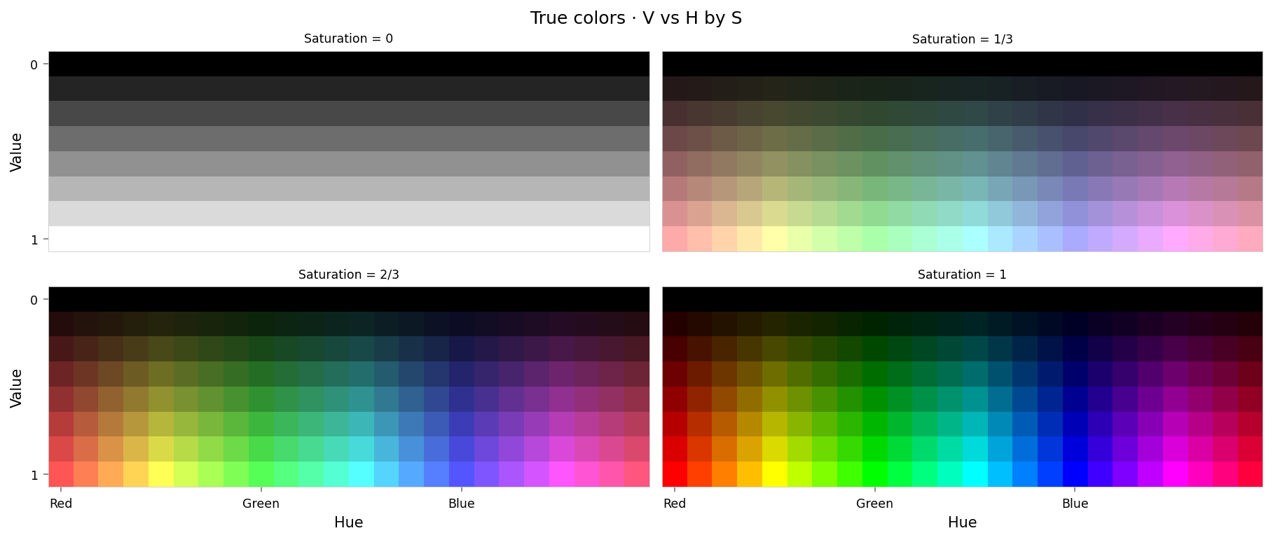
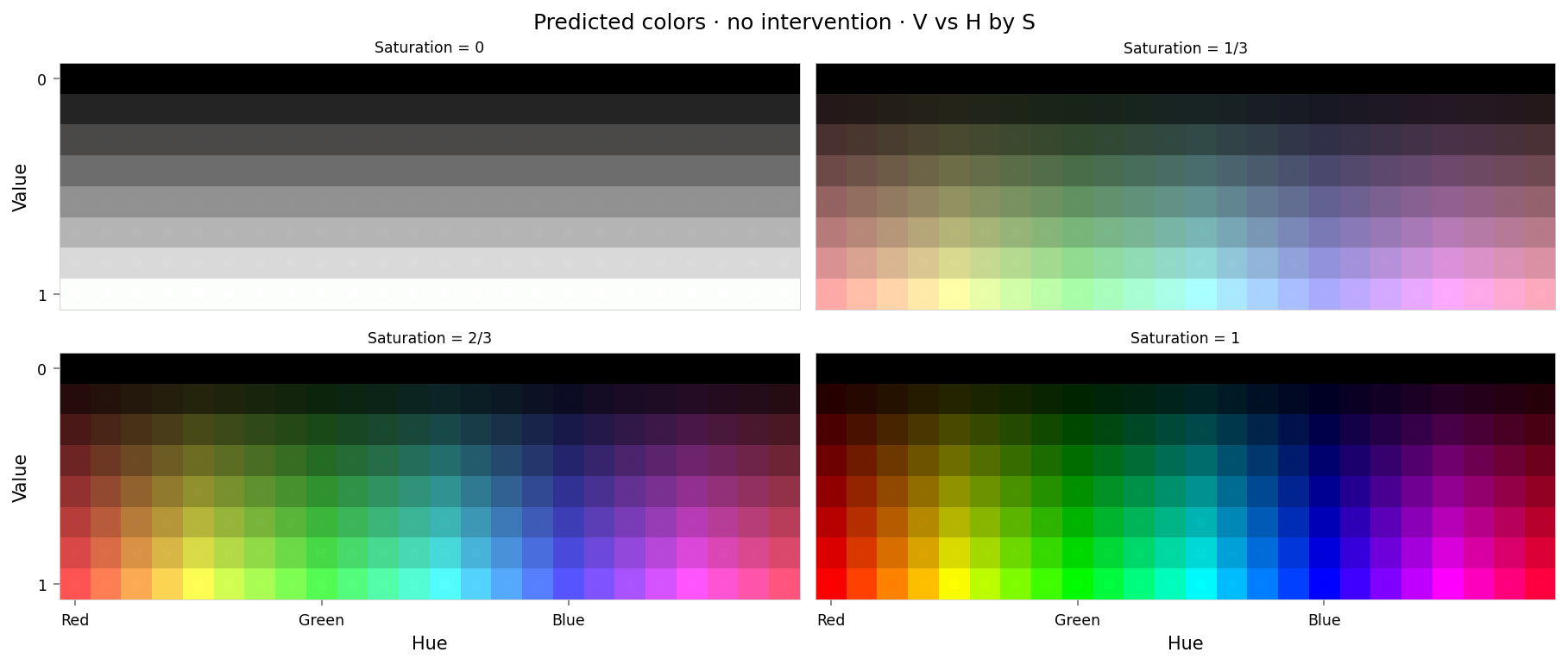
Quick sense-check: Let's see how well the trained model reconstructs colors.
from IPython.display import clear_output

import importlib
import utils.nb
import utils.plt

importlib.reload(utils.nb)
importlib.reload(utils.plt)

from ex_color.vis import plot_colors
from utils.nb import displayer_mpl


hsv_cube = ColorCube.from_hsv(
    h=arange_cyclic(step_size=1 / 24),
    s=np.linspace(0, 1, 4),
    v=np.linspace(0, 1, 8),
).permute('svh')
x_hsv = torch.tensor(hsv_cube.rgb_grid, dtype=torch.float32)

hd_hsv_cube = ColorCube.from_hsv(
    h=arange_cyclic(step_size=1 / 240),
    s=np.linspace(0, 1, 48),
    v=np.linspace(0, 1, 48),
)
hd_x_hsv = torch.tensor(hd_hsv_cube.rgb_grid, dtype=torch.float32)

rgb_cube = ColorCube.from_rgb(
    r=np.linspace(0, 1, 20),
    g=np.linspace(0, 1, 20),
    b=np.linspace(0, 1, 20),
)
x_rgb = torch.tensor(rgb_cube.rgb_grid, dtype=torch.float32)

with displayer_mpl(
    f'large-assets/ex-{nbid}-true-colors.png',
    alt_text="""Plot showing four slices of the HSV cube, titled "{title}". Each slice has constant saturation, but varies in value (brightness) from top to bottom, and in hue from left to right. The first slice shows a grayscale gradient from black to white; the last shows the fully-saturated color spectrum.""",
) as show:
    show(lambda: plot_colors(hsv_cube, title='True colors', colors=x_hsv.numpy()))
from IPython.display import clear_output
from torch.nn import functional as F

from ex_color.vis import plot_colors, plot_cube_series


interventions = []
y_hsv = await infer(model, x_hsv)
hd_y_hsv = await infer(model, hd_x_hsv)
clear_output()

with displayer_mpl(
    f'large-assets/ex-{nbid}-pred-colors-no-intervention.png',
    alt_text="""Plot showing four slices of the HSV cube, titled "{title}". Nominally, each slice has constant saturation, but varies in value (brightness) from top to bottom, and in hue from left to right. Each color value is represented as a square patch of that color. The outer portion of the patches shows the color as reconstructed by the model; the inner portion shows the true (input) color. The reconstructed and true colors agree fairly well, but some slight differences are visible; for example, "white" is slightly gray, and many of the fully-saturated colors are less saturated than they should be.""",
) as show:
    show(
        lambda: plot_colors(
            hsv_cube,
            title='Predicted colors · no intervention',
            colors=y_hsv.numpy(),
            colors_compare=x_hsv.numpy(),
        )
    )

per_color_loss = F.mse_loss(hd_y_hsv, hd_x_hsv, reduction='none').mean(dim=-1)
loss_cube = hd_hsv_cube.assign('MSE', per_color_loss.numpy().reshape(hd_hsv_cube.shape))
max_loss = per_color_loss.max().item()
median_loss = per_color_loss.median().item()

with displayer_mpl(
    f'large-assets/ex-{nbid}-loss-colors-no-intervention.png',
    alt_text=f"""Line chart showing loss per color, titled "{{title}}". Y-axis: mean square error, ranging from zero to {max_loss:.2g}. X-axis: hue. The range of loss values is small, but there are two notable peaks at red, yellow, green, and cyan. Between those points the lines are wavy, reminiscent of an audio waveform.""",
) as show:
    show(
        lambda: plot_cube_series(
            loss_cube.permute('hsv')[:, -1:, :: (loss_cube.shape[2] // -5)],
            loss_cube.permute('svh')[:, -1:, :: -(loss_cube.shape[0] // -3)],
            loss_cube.permute('vsh')[:, -1:, :: -(loss_cube.shape[0] // -3)],
            title='Reconstruction error · no intervention',
            var='MSE',
            figsize=(12, 3),
        )
    )
print(f'Max loss: {max_loss:.2g}')
print(f'Median MSE: {median_loss:.2g}')

Max loss: 0.00019
Median MSE: 8.1e-06
Reconstruction loss looks good in that it's low — but the curves are pretty wiggly. That probably means latent space is a bit lumpy on small scales.
# # Generate a list of dimensions to visualize
# from itertools import combinations
# [
#     (
#         b,
#         a,
#         (a + 1) % 5 if (a + 1) % 5 not in (a, b) else (a + 2) % 5,
#     )
#     for a, b in combinations((0, 1, 2, 3, 4), 2)
# ]
from IPython.display import clear_output

from ex_color.vis import plot_latent_grid_3d

y_rgb, h_rgb = await infer_with_latent_capture(model, x_rgb, 'bottleneck')
clear_output()

with displayer_mpl(
    f'large-assets/ex-{nbid}-latents-no-intervention.png',
    alt_text="""Two rows of three spherical plots, titled "{title}". Each plot shows a vibrant collection of colored circles or balls scattered over the surface of a sphere. On the top row, the first plot shows a thick curve — like a tongue seen from the side — touching the top and right side of the sphere and passing through the middle. It is red at the top, purple and blue in the middle, and cyan on the right. The sphere is empty elsewhere. The other plots in the top row show different views of the same space, all with red at the top but a different horizontal axis. They look much more dome-shaped. The second row shows still more views, focused on the other dimensions. These are more spherical and almost look like color wheels, but with the colors out of order.""",
) as show:
    show(
        lambda theme: plot_latent_grid_3d(
            h_rgb,
            y_rgb,
            x_rgb,
            title='Latents · no intervention',
            dims=[
                (1, 0, 2),
                (2, 0, 1),
                (3, 0, 1),
                # (4, 0, 1),
                # (2, 1, 3),
                # (3, 1, 2),
                (4, 1, 2),
                (3, 2, 4),
                # (4, 2, 3),
                (4, 3, 0),
            ],
            dot_radius=10,
            theme=theme,
        )
    )
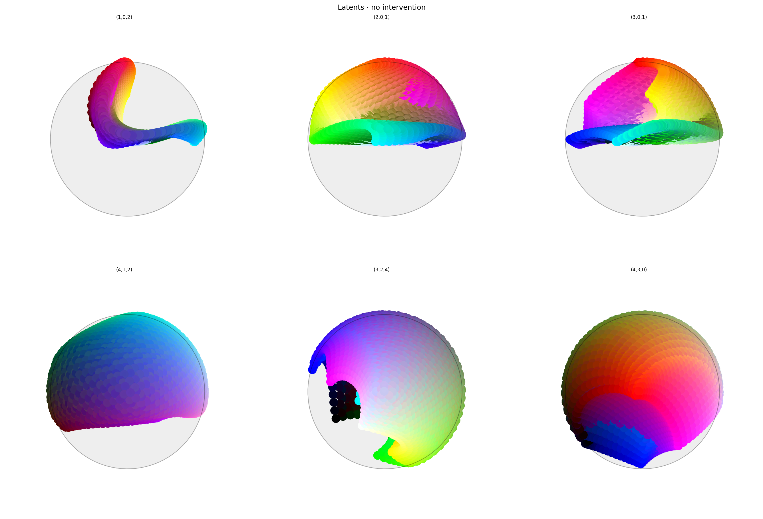
Latent space looks promising: the first two dimensions show a shape with a thin, flat base and red colors rising to the anchor point. This is similar to what I expected to see, although I expected it to have a symmetrical base.
Apart from that interesting shape, the structure looks similar to the one in 2.8.
Let's see what happens when we ablate the first dimension.
Ablation
Now that we have our model, let's try ablating (zeroing) hue. We'll use the same function as 2.8.
def ablate[M](model: M, layer_id: str, dims: Sequence[int]) -> M:
    """Return a copy of model where the selected latent dims are effectively nulled."""
    ...
This zeros out producer (upstream matrix) rows and consumer (downstream) columns for the given dims. Shapes remain unchanged.
from ex_color.surgery import ablate

ablated_model = ablate(model, 'bottleneck', [0])

y_hsv = await infer(ablated_model, x_hsv)
hd_y_hsv = await infer(ablated_model, hd_x_hsv)
clear_output()

with displayer_mpl(
    f'large-assets/ex-{nbid}-pred-colors-ablated.png',
    alt_text="""Plot showing four slices of the HSV cube, titled "{title}". Nominally, each slice has constant saturation, but varies in value (brightness) from top to bottom, and in hue from left to right. Each color value is represented as a square patch of that color. The outer portion of the patches shows the color as reconstructed by the model; the inner portion shows the true (input) color. The reconstructed and true colors agree fairly well up to yellow and purple, but disagree significantly near red. Desaturated colors and grays are almost unchanged.""",
) as show:
    show(
        lambda: plot_colors(
            hsv_cube,
            title='Predicted colors · ablated',
            colors=y_hsv.numpy(),
            colors_compare=x_hsv.numpy(),
        )
    )

per_color_loss = F.mse_loss(hd_y_hsv, hd_x_hsv, reduction='none').mean(dim=-1)
loss_cube = hd_hsv_cube.assign('MSE', per_color_loss.numpy().reshape(hd_hsv_cube.shape))
max_loss = per_color_loss.max().item()
median_loss = per_color_loss.median().item()
with displayer_mpl(
    f'large-assets/ex-{nbid}-loss-colors-ablated.png',
    alt_text=f"""Line chart showing loss per color, titled "{{title}}". Y-axis: mean square error, ranging from zero to {max_loss:.2g}. X-axis: hue. There is very low error at yellow-green, green, cyan, blue, and purple; high error at red, and moderate error at yellow and magenta. Saturation and value show low error at white and black, with error levels gradually increasing toward vibrant red. The curves are fairly smooth, but show a high-frequency dip very close to red. In fact red-orange has higher error than pure red.""",
) as show:
    show(
        lambda: plot_cube_series(
            loss_cube.permute('hsv')[:, -1:, :: (loss_cube.shape[2] // -5)],
            loss_cube.permute('svh')[:, -1:, :: -(loss_cube.shape[0] // -6)],
            loss_cube.permute('vsh')[:, -1:, :: -(loss_cube.shape[0] // -6)],
            title='Reconstruction error · ablated',
            var='MSE',
            figsize=(12, 3),
        )
    )
print(f'Max loss: {max_loss:.2g}')
print(f'Median MSE: {median_loss:.2g}')

Max loss: 0.26
Median MSE: 0.00014
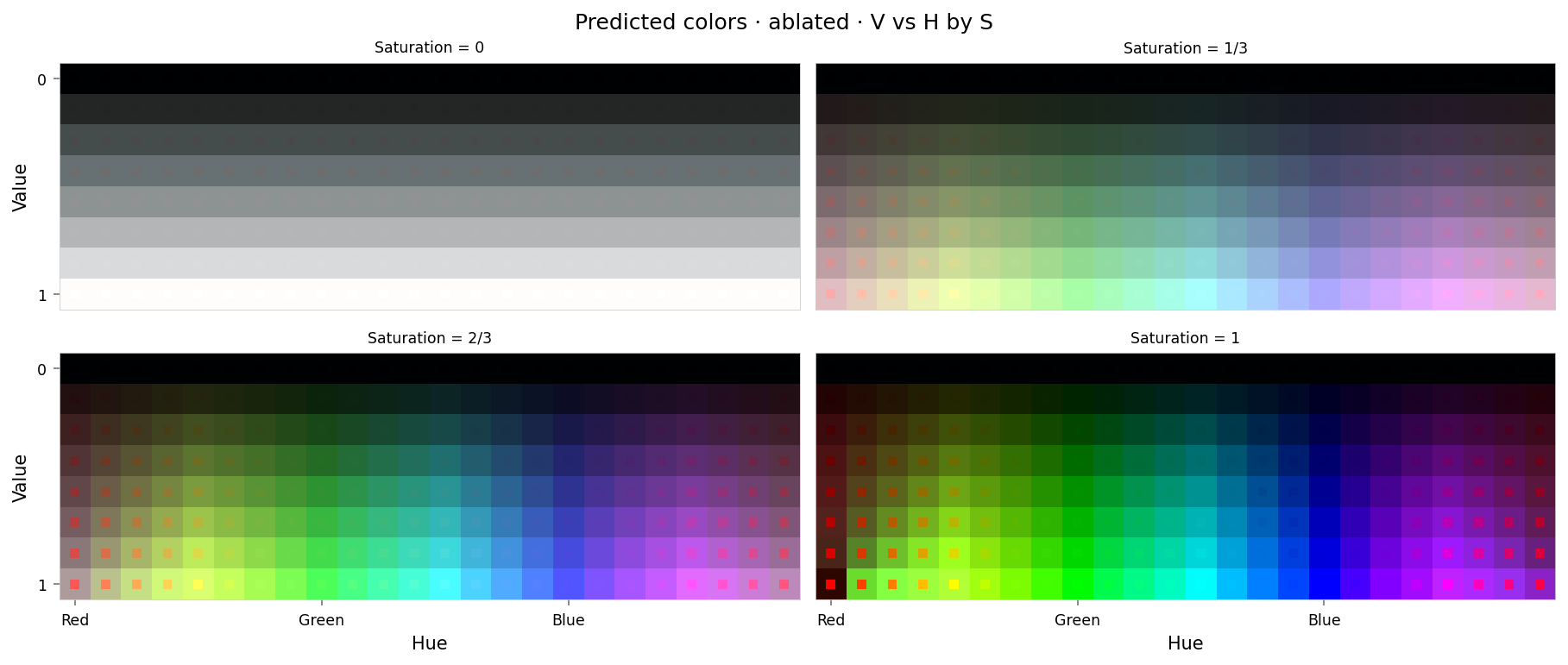
This looks like a fairly clean ablation: similar to Ex 2.6, but without any affect on cyan. The error curves near red are similar in magnitude to those in 2.6, but not as clean: there are some high-frequency bumps close to red, and in fact orange-red has the highest error. But this is a much better result than Ex 2.8: the ablation has only affected red, similarly to the directional interventions of Ex 2.4.
from IPython.display import clear_output

from ex_color.vis import plot_latent_grid_3d

y_rgb, h_rgb = await infer_with_latent_capture(ablated_model, x_rgb, 'bottleneck')
clear_output()

with displayer_mpl(
    f'large-assets/ex-{nbid}-latents-ablated.png',
    alt_text="""Two rows of three spherical plots, titled "{title}". Each plot shows a vibrant collection of colored circles or balls scattered over the surface of a sphere. The vertical axis of each plot in the top row is the first dimension of latent space. The plots in the top row all have a line across the equator varying between purple, blue, green, and white. The bottom row shows similar colors, but with more of a ball-like appearance. Each circle has a point in the middle showing the true color of the sample; the bottom row shows that many of the warmer colors have been shifted to purple or black.""",
) as show:
    show(
        lambda theme: plot_latent_grid_3d(
            h_rgb,
            y_rgb,
            x_rgb,
            title='Latents · ablated',
            dims=[
                (1, 0, 2),
                (2, 0, 1),
                (3, 0, 1),
                # (4, 0, 1),
                # (2, 1, 3),
                # (3, 1, 2),
                (4, 1, 2),
                (3, 2, 4),
                # (4, 2, 3),
                (4, 3, 0),
            ],
            dot_radius=10,
            theme=theme,
        )
    )
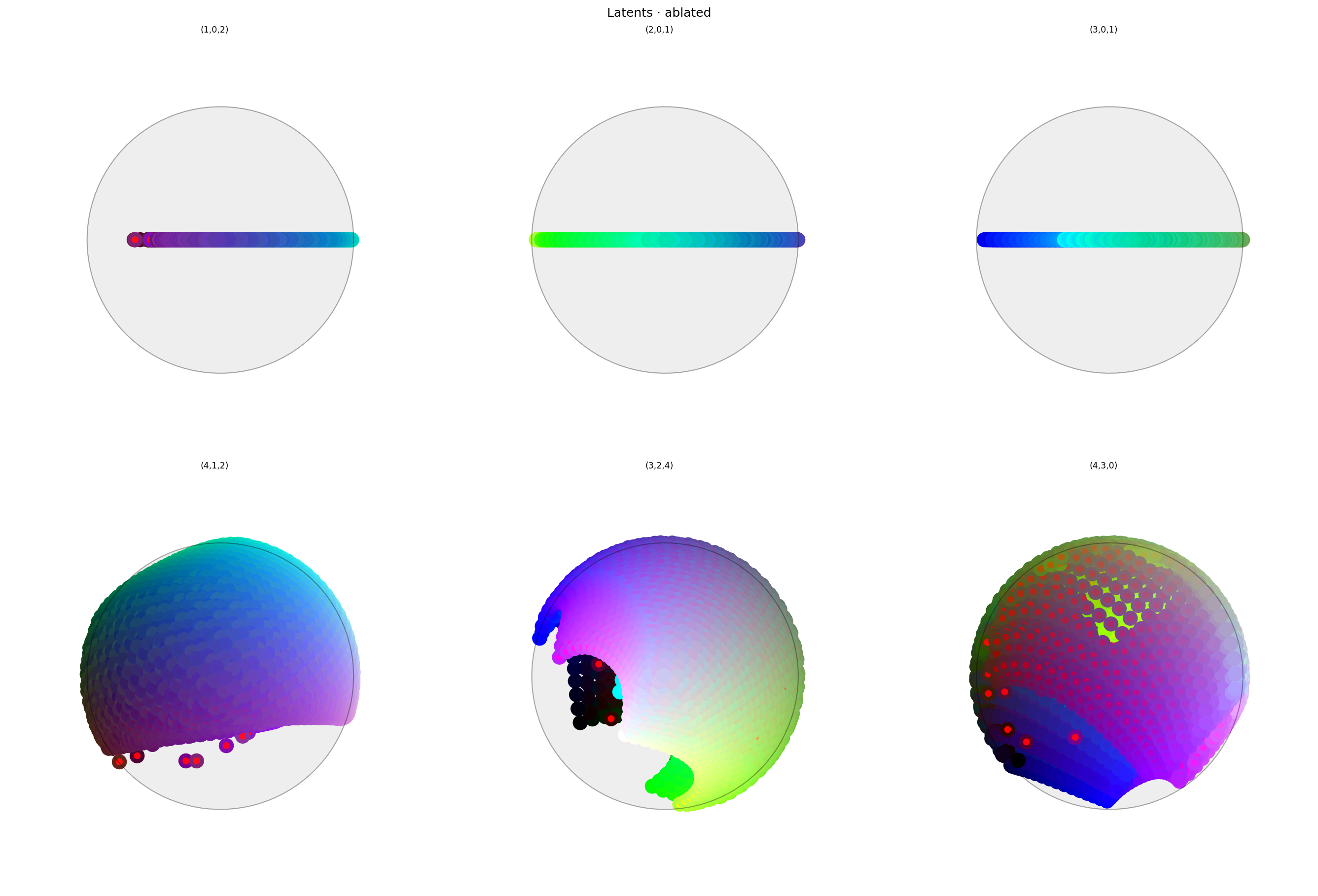
Here we clearly see that the first dimension has been removed from latent space, but it's hard to say what else has happened. I think maybe the space is now so high-dimensional that it's becoming hard to interpret.
Conclusion
Hypothesis confirmed: adding another dimension to the bottleneck and an extra nonlinearity to the encoder and decoder has given the model the capacity it needed to satisfy the constraints, including the new anti-anchor regularization term. Latent space has been warped in such a way that only colors close to red are in the first dimension, allowing that concept to be cleanly ablated.