Experiment 2.8: Delete only red
In Ex 2.6, we demonstrated that we could delete a single axis: warmth (red-cyan). That happened to be possible because we had regularized the model such that warmth was axis-aligned¹. And in Ex 2.4, we showed that red could be intervened on without affecting other colors (not even cyan, which shares an axis). In this experiment, we'll see if we can delete red without also deleting cyan. This is trickier than the earlier experiments, because our deletion mechanisms affect entire dimensions, not just the positive direction.
Hypothesis
If we add a regularizer to push colors away from being opposed to red, then when we delete the red dimension, other colors should be mostly unaffected.
¹ Although warmth is isolated to a single dimension, I'm not sure if it's right to say that it's monosemantic: it's part of a linear space that happens to be axis-aligned.
from __future__ import annotations

nbid = '2.8'  # ID for tagging assets
nbname = 'Ablate red (only)'
experiment_name = f'Ex {nbid}: {nbname}'
project = 'ex-preppy'
# Basic setup: Logging, Experiment (Modal)
import logging

import modal

from infra.requirements import freeze, project_packages
from mini.experiment import Experiment
from utils.logging import SimpleLoggingConfig

logging_config = (
    SimpleLoggingConfig()
    .info('notebook', 'utils', 'mini', 'ex_color')
    .error('matplotlib.axes')  # Silence warnings about set_aspect
)
logging_config.apply()

# This is the logger for this notebook
log = logging.getLogger(f'notebook.{nbid}')

run = Experiment(experiment_name, project=project)
run.image = modal.Image.debian_slim().pip_install(*freeze(all=True)).add_local_python_source(*project_packages())
run.before_each(logging_config.apply)
None  # prevent auto-display of this cell
Regularizers
Like Ex 2.6:
- Anchor: pins
redto $(1,0,0,0)$. - Separate: angular repulsion to reduce global clumping (applied within each batch).
- Unitarity: pulls all embeddings to the surface of the unit hypersphere, i.e. it makes the embedding vectors have unit length.
But unlike earlier experiments:
- Anti-anchor: repels everything from $(-1,0,0,0)$.
- Anchor: has been switched to angular repulsion instead of Euclidean. The new regularizer operates similarly to separate: it encourages high cosine similarity; but it compares samples to a fixed point rather than other samples in the batch. This seems to have minimal effect, but it seems more principled.
- No planarity: to maximize the freedom to place hues in other dimensions, the planarity constraint is removed.
import torch

from mini.temporal.dopesheet import Dopesheet
from ex_color.loss import AngularAnchor, AntiAnchor, Separate, Unitarity, RegularizerConfig

from ex_color.training import TrainingModule

K = 4  # bottleneck dimensionality
RED = (1, 0, 0, 0)
ANTI_RED = tuple(-c for c in RED)
assert len(RED) == len(ANTI_RED) == K

ALL_REGULARIZERS = [
    RegularizerConfig(
        name='reg-unit',
        compute_loss_term=Unitarity(),
        label_affinities=None,
        layer_affinities=['encoder'],
    ),
    RegularizerConfig(
        name='reg-anchor',
        compute_loss_term=AngularAnchor(torch.tensor(RED, dtype=torch.float32)),
        label_affinities={'red': 1.0},
        layer_affinities=['bottleneck'],
    ),
    RegularizerConfig(
        name='reg-separate',
        compute_loss_term=Separate(power=100.0, shift=True),
        label_affinities=None,
        layer_affinities=['bottleneck'],
    ),
    RegularizerConfig(
        name='reg-anti-anchor',
        compute_loss_term=AntiAnchor(torch.tensor(ANTI_RED, dtype=torch.float32)),
        label_affinities=None,
        layer_affinities=['bottleneck'],
    ),
]
from functools import partial
from torch import Tensor
from torch.utils.data import DataLoader, TensorDataset, WeightedRandomSampler
import numpy as np

from ex_color.data.color_cube import ColorCube
from ex_color.data.cube_sampler import vibrancy
from ex_color.data.cyclic import arange_cyclic
from ex_color.labelling import collate_with_generated_labels


def prep_data() -> tuple[DataLoader, Tensor]:
    """
    Prepare data for training.

    Returns: (train, val)
    """
    hsv_cube = ColorCube.from_hsv(
        h=arange_cyclic(step_size=10 / 360),
        s=np.linspace(0, 1, 10),
        v=np.linspace(0, 1, 10),
    )
    hsv_tensor = torch.tensor(hsv_cube.rgb_grid.reshape(-1, 3), dtype=torch.float32)
    vibrancy_tensor = torch.tensor(vibrancy(hsv_cube).flatten(), dtype=torch.float32)
    hsv_dataset = TensorDataset(hsv_tensor, vibrancy_tensor)

    labeller = partial(
        collate_with_generated_labels,
        soft=False,  # Use binary labels (stochastic) to simulate the labelling of internet text
        red=0.5,
        vibrant=0.5,
        desaturated=0.5,
    )
    # Desaturated and dark colors are over-represented in the cube, so we use a weighted sampler to balance them out
    hsv_loader = DataLoader(
        hsv_dataset,
        batch_size=64,
        num_workers=2,
        sampler=WeightedRandomSampler(
            weights=hsv_cube.bias.flatten().tolist(),
            num_samples=len(hsv_dataset),
            replacement=True,
        ),
        collate_fn=labeller,
    )

    rgb_cube = ColorCube.from_rgb(
        r=np.linspace(0, 1, 8),
        g=np.linspace(0, 1, 8),
        b=np.linspace(0, 1, 8),
    )
    rgb_tensor = torch.tensor(rgb_cube.rgb_grid.reshape(-1, 3), dtype=torch.float32)
    return hsv_loader, rgb_tensor
import wandb
from ex_color.model import CNColorMLP


# @run.thither(env={'WANDB_API_KEY': wandb.Api().api_key})
async def train(
    dopesheet: Dopesheet,
    regularizers: list[RegularizerConfig],
    k_bottleneck: int,
) -> CNColorMLP:
    """Train the model with the given dopesheet and variant."""
    import lightning as L
    from lightning.pytorch.loggers import WandbLogger

    from ex_color.seed import set_deterministic_mode

    from utils.progress.lightning import LightningProgress

    log.info(f'Training with: {[r.name for r in regularizers]}')

    seed = 0
    set_deterministic_mode(seed)

    hsv_loader, _ = prep_data()

    model = CNColorMLP(k_bottleneck)
    total_params = sum(p.numel() for p in model.parameters() if p.requires_grad)
    log.debug(f'Model initialized with {total_params:,} trainable parameters.')

    training_module = TrainingModule(model, dopesheet, torch.nn.MSELoss(), regularizers)

    logger = WandbLogger(experiment_name, project=project)

    trainer = L.Trainer(
        max_steps=len(dopesheet),
        callbacks=[
            LightningProgress(),
        ],
        enable_checkpointing=False,
        enable_model_summary=False,
        # enable_progress_bar=True,
        logger=logger,
    )

    print(f'max_steps: {len(dopesheet)}, hsv_loader length: {len(hsv_loader)}')

    # Train the model
    try:
        trainer.fit(training_module, hsv_loader)
    finally:
        wandb.finish()
    # This is only a small model, so it's OK to return it rather than storing and loading a checkpoint remotely
    return model


async with run():
    model = await train(Dopesheet.from_csv(f'./ex-{nbid}-dopesheet.csv'), ALL_REGULARIZERS, K)
I 574.5 no.2.8:Training with: ['reg-unit', 'reg-anchor', 'reg-separate', 'reg-anti-anchor']
INFO: Seed set to 0
I 574.5 li.fa.ut.se:Seed set to 0
I 574.5 ex.se: PyTorch set to deterministic mode
INFO: GPU available: False, used: False
I 574.5 li.py.ut.ra:GPU available: False, used: False
INFO: TPU available: False, using: 0 TPU cores
I 574.5 li.py.ut.ra:TPU available: False, using: 0 TPU cores
INFO: HPU available: False, using: 0 HPUs
I 574.5 li.py.ut.ra:HPU available: False, using: 0 HPUs
max_steps: 3001, hsv_loader length: 57
./wandb/run-20250907_031727-058nuvr4
Starting phase: Train
INFO: `Trainer.fit` stopped: `max_steps=3001` reached.
I 592.9 li.py.ut.ra:`Trainer.fit` stopped: `max_steps=3001` reached.
Run history:
| epoch | ▁▁▁▁▂▂▂▂▂▂▃▃▃▄▄▄▄▄▄▅▅▅▅▅▅▆▆▆▆▆▇▇▇▇▇▇████ |
| train_loss | █▄▆▃▃▄▃▂▃▂▂▄▃▃▂▂▂▂▂▂▂▂▂▂▁▁▁▁▁▁▁▁▁▁▁▁▁▁▁▁ |
| train_recon | █▂▂▂▁▁▁▁▁▁▁▁▁▂▁▁▁▁▁▁▁▁▁▁▁▁▁▁▁▁▁▁▁▁▁▁▁▁▁▁ |
| train_reg-anchor | ▁▁█▁▁▄▁▁▁▁▁▁▃▁▁▁▁▁▁▁▁▁▁▁▁▁▁▁▁▁▁▁▁▁▁▁▁▁▁▁ |
| train_reg-anti-anchor | ▇▁▁▁▁▂▅▄▁▁▁▅▆▁▁▁▁▁▃▂▁▂▄█▃▁▁▃▁▁▁▁▂▃▂▂▁▂▁▁ |
| train_reg-separate | █▇█▆▇▅▄▇▅▇▅▄▄▄▇▅▆▃▂▂▁▃▁▃▄▃▃▃▂▄▃▄▃▄▃▃▄▇▄▅ |
| train_reg-unit | █▇▆▅▃▁▁▁▁▁▁▁▁▁▁▁▁▁▁▁▁▁▁▁▁▁▁▁▁▁▁▁▁▁▁▁▁▁▁▁ |
| trainer/global_step | ▁▁▁▁▁▂▂▂▂▂▂▃▃▃▃▃▃▄▄▄▄▄▄▅▅▅▅▅▅▅▆▆▆▆▇▇▇███ |
Run summary:
| epoch | 52 |
| train_loss | 2e-05 |
| train_recon | 2e-05 |
| train_reg-anchor | 0.02208 |
| train_reg-anti-anchor | 0 |
| train_reg-separate | 0.48801 |
| train_reg-unit | 0.00507 |
| trainer/global_step | 2999 |
View project at: https://wandb.ai/z0r/ex-color-transformer
Synced 5 W&B file(s), 0 media file(s), 0 artifact file(s) and 0 other file(s)
./wandb/run-20250907_031727-058nuvr4/logs
The charts training look OK.
The anti-anchor term maintained fairly high loss to the end — which probably means that it wasn't successful in pushing points away from the anchor point.
from ex_color.inference import InferenceModule


async def infer(
    model: CNColorMLP,
    test_data: Tensor,
) -> Tensor:
    """Run inference with the given model."""
    import lightning as L

    inference_module = InferenceModule(model, [])
    trainer = L.Trainer(
        enable_checkpointing=False,
        enable_model_summary=False,
        enable_progress_bar=True,
    )
    reconstructed_colors_batches = trainer.predict(
        inference_module,
        DataLoader(
            TensorDataset(test_data.reshape((-1, 3))),
            batch_size=64,
            collate_fn=lambda batch: torch.stack([row[0] for row in batch], 0),
        ),
    )
    assert reconstructed_colors_batches is not None
    # Flatten the list of batches to a single list of tensors
    reconstructed_colors = [item for batch in reconstructed_colors_batches for item in batch]
    # Reshape to match input
    return torch.cat(reconstructed_colors).reshape(test_data.shape)
import torch
import numpy as np

from ex_color.inference import InferenceModule


async def infer_with_latent_capture(
    model: CNColorMLP,
    test_data: Tensor,
    layer_name: str = 'bottleneck',
) -> tuple[Tensor, Tensor]:
    module = InferenceModule(model, [], capture_layers=[layer_name])
    import lightning as L

    trainer = L.Trainer(enable_checkpointing=False, enable_model_summary=False, enable_progress_bar=False)
    batches = trainer.predict(
        module,
        DataLoader(
            TensorDataset(test_data.reshape((-1, 3))),
            batch_size=64,
            collate_fn=lambda batch: torch.stack([row[0] for row in batch], 0),
        ),
    )
    assert batches is not None
    preds = [item for batch in batches for item in batch]
    y = torch.cat(preds).reshape(test_data.shape)
    # Read captured activations as a flat [N, D] tensor
    latents = module.read_captured(layer_name)
    return y, latents
Quick sense-check: Let's see how well the trained model reconstructs colors.
from IPython.display import clear_output

import importlib
import utils.nb
import utils.plt

importlib.reload(utils.nb)
importlib.reload(utils.plt)

from ex_color.vis import plot_colors
from utils.nb import displayer_mpl


hsv_cube = ColorCube.from_hsv(
    h=arange_cyclic(step_size=1 / 24),
    s=np.linspace(0, 1, 4),
    v=np.linspace(0, 1, 8),
).permute('svh')
x_hsv = torch.tensor(hsv_cube.rgb_grid, dtype=torch.float32)

hd_hsv_cube = ColorCube.from_hsv(
    h=arange_cyclic(step_size=1 / 240),
    s=np.linspace(0, 1, 48),
    v=np.linspace(0, 1, 48),
)
hd_x_hsv = torch.tensor(hd_hsv_cube.rgb_grid, dtype=torch.float32)

rgb_cube = ColorCube.from_rgb(
    r=np.linspace(0, 1, 20),
    g=np.linspace(0, 1, 20),
    b=np.linspace(0, 1, 20),
)
x_rgb = torch.tensor(rgb_cube.rgb_grid, dtype=torch.float32)

with displayer_mpl(
    f'large-assets/ex-{nbid}-true-colors.png',
    alt_text="""Plot showing four slices of the HSV cube, titled "{title}". Each slice has constant saturation, but varies in value (brightness) from top to bottom, and in hue from left to right. The first slice shows a grayscale gradient from black to white; the last shows the fully-saturated color spectrum.""",
) as show:
    show(lambda: plot_colors(hsv_cube, title='True colors', colors=x_hsv.numpy()))
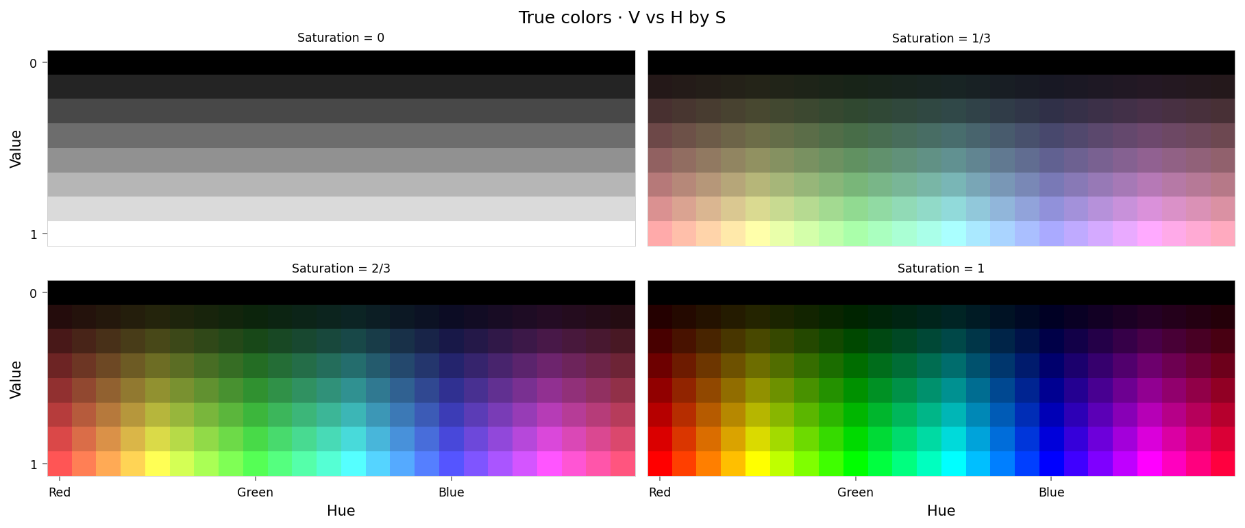
from IPython.display import clear_output
from torch.nn import functional as F

from ex_color.vis import plot_colors, plot_cube_series


interventions = []
y_hsv = await infer(model, x_hsv)
hd_y_hsv = await infer(model, hd_x_hsv)
clear_output()

with displayer_mpl(
    f'large-assets/ex-{nbid}-pred-colors-no-intervention.png',
    alt_text="""Plot showing four slices of the HSV cube, titled "{title}". Nominally, each slice has constant saturation, but varies in value (brightness) from top to bottom, and in hue from left to right. Each color value is represented as a square patch of that color. The outer portion of the patches shows the color as reconstructed by the model; the inner portion shows the true (input) color. The reconstructed and true colors agree fairly well, but some slight differences are visible; for example, "white" is slightly gray, and many of the fully-saturated colors are less saturated than they should be.""",
) as show:
    show(
        lambda: plot_colors(
            hsv_cube,
            title='Predicted colors · no intervention',
            colors=y_hsv.numpy(),
            colors_compare=x_hsv.numpy(),
        )
    )

per_color_loss = F.mse_loss(hd_y_hsv, hd_x_hsv, reduction='none').mean(dim=-1)
loss_cube = hd_hsv_cube.assign('MSE', per_color_loss.numpy().reshape(hd_hsv_cube.shape))
max_loss = per_color_loss.max().item()
median_loss = per_color_loss.median().item()

with displayer_mpl(
    f'large-assets/ex-{nbid}-loss-colors-no-intervention.png',
    alt_text=f"""Line chart showing loss per color, titled "{{title}}". Y-axis: mean square error, ranging from zero to {max_loss:.2g}. X-axis: hue. The range of loss values is small, but there are two notable peaks at all primary and secondary colors (red, yellow, green, etc.), and at black and white.""",
) as show:
    show(
        lambda: plot_cube_series(
            loss_cube.permute('hsv')[:, -1:, :: (loss_cube.shape[2] // -5)],
            loss_cube.permute('svh')[:, -1:, :: -(loss_cube.shape[0] // -3)],
            loss_cube.permute('vsh')[:, -1:, :: -(loss_cube.shape[0] // -3)],
            title='Reconstruction error · no intervention',
            var='MSE',
            figsize=(12, 3),
        )
    )
print(f'Max loss: {max_loss:.2g}')
print(f'Median MSE: {median_loss:.2g}')
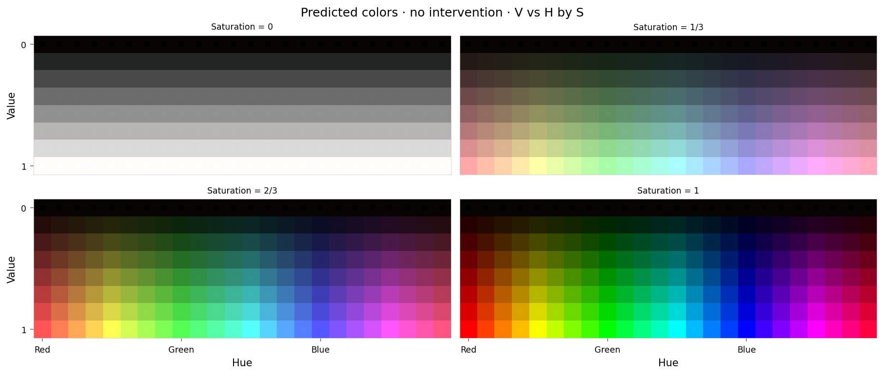

Max loss: 0.00048
Median MSE: 1.1e-05
from IPython.display import clear_output

from ex_color.vis import plot_latent_grid_3d

y_rgb, h_rgb = await infer_with_latent_capture(model, x_rgb, 'bottleneck')
clear_output()

with displayer_mpl(
    f'large-assets/ex-{nbid}-latents-no-intervention.png',
    alt_text="""Two rows of three spherical plots, titled "{title}". Each plot shows a vibrant collection of colored circles or balls scattered over the surface of a sphere. On the top row, the first plot is hemispherical, like a helmet, with red at the top, cyan or white at the side, and green in the middle. The lower half of the sphere is mostly empty but some colors extend beyond the equator. The other plots show different views of the same space, all with red at the top but a different horizontal axis. The second row show still more views, focused on the other dimensions. These are more spherical and almost look like color wheels, but with the colors out of order.""",
) as show:
    show(
        lambda theme: plot_latent_grid_3d(
            h_rgb,
            y_rgb,
            x_rgb,
            title='Latents · no intervention',
            dims=[
                (1, 0, 2),
                (2, 0, 1),
                (3, 0, 2),
                (1, 2, 0),
                (1, 3, 0),
                (2, 3, 1),
            ],
            dot_radius=10,
            theme=theme,
        )
    )
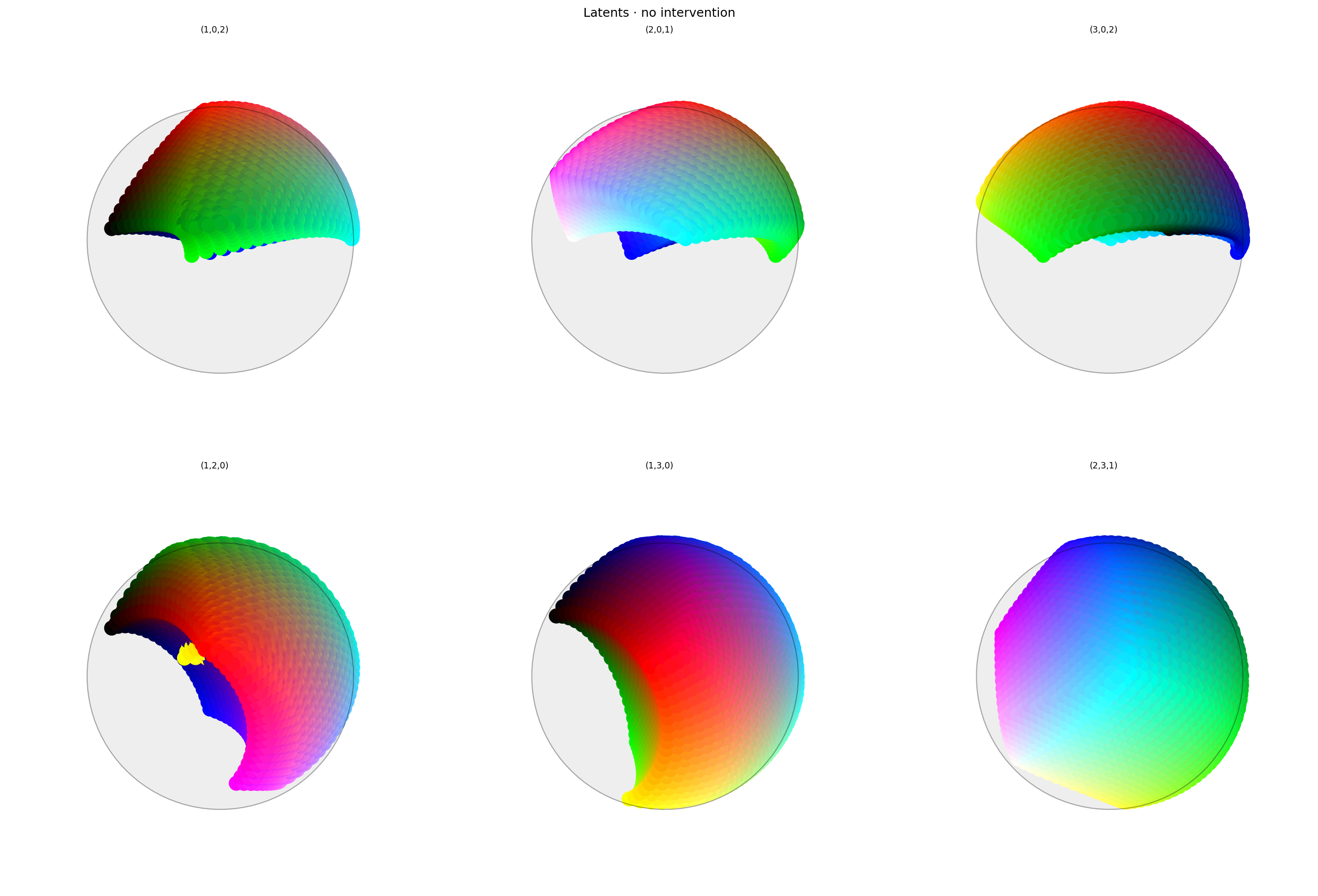
Latent space looks OK. As expected, red has been positioned at $(1,0,0,0)$ but there is nothing opposite it.
There are a lot of colors in the red hemi-hypersphere (positive $0$): various pinks, greys, and greens. That's probably to be expected: everything is being repelled from opposing red and it has to go somewhere. But it may cause problems when we delete the first dimension.
Ablation
Now that we have our model, let's try ablating (zeroing) red. We'll use the same function as 2.6.
def ablate[M](model: M, layer_id: str, dims: Sequence[int]) -> M:
    """Return a copy of model where the selected latent dims are effectively nulled."""
    ...
This zeros out producer (upstream matrix) rows and consumer (downstream) columns for the given dims. Shapes remain unchanged.
We'll delete the whole first dimesion.
from ex_color.surgery import ablate

ablated_model = ablate(model, 'bottleneck', [0])

y_hsv = await infer(ablated_model, x_hsv)
hd_y_hsv = await infer(ablated_model, hd_x_hsv)
clear_output()

with displayer_mpl(
    f'large-assets/ex-{nbid}-pred-colors-ablated.png',
    alt_text="""Plot showing four slices of the HSV cube, titled "{title}". Nominally, each slice has constant saturation, but varies in value (brightness) from top to bottom, and in hue from left to right. The slices don't look right at all: black and white are correct, but all other grays are much too bright. The saturated slices do resemble a spectrum, but only green and blue are present and they look washed out.""",
) as show:
    show(
        lambda: plot_colors(
            hsv_cube,
            title='Predicted colors · ablated',
            colors=y_hsv.numpy(),
            colors_compare=x_hsv.numpy(),
        )
    )

per_color_loss = F.mse_loss(hd_y_hsv, hd_x_hsv, reduction='none').mean(dim=-1)
loss_cube = hd_hsv_cube.assign('MSE', per_color_loss.numpy().reshape(hd_hsv_cube.shape))
max_loss = per_color_loss.max().item()
median_loss = per_color_loss.median().item()
with displayer_mpl(
    f'large-assets/ex-{nbid}-loss-colors-ablated.png',
    alt_text=f"""Line chart showing loss per color, titled "{{title}}". Y-axis: mean square error, ranging from zero to {max_loss:.2g}. X-axis: hue. There is indeed low error at cyan and high error at red — but there is also some error at yellow, magenta, and at the mid-tones of both saturation and value.""",
) as show:
    show(
        lambda: plot_cube_series(
            loss_cube.permute('hsv')[:, -1:, :: (loss_cube.shape[2] // -5)],
            loss_cube.permute('svh')[:, -1:, :: -(loss_cube.shape[0] // -6)],
            loss_cube.permute('vsh')[:, -1:, :: -(loss_cube.shape[0] // -6)],
            title='Reconstruction error · ablated',
            var='MSE',
            figsize=(12, 3),
        )
    )
print(f'Max loss: {max_loss:.2g}')
print(f'Median MSE: {median_loss:.2g}')
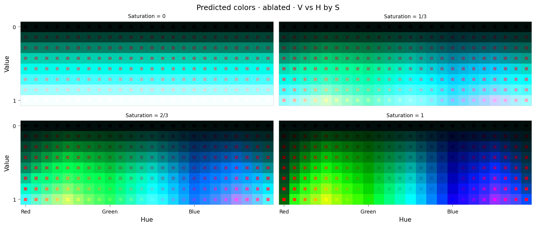

Max loss: 0.74
Median MSE: 0.044
That looks really bad. At first glance the loss curves aren't too bad, but the cube slices look completely different — so our ablation hasn't been limited to red at all. Looking again the loss curves, although cyan has low error, there is moderate error at yellow, magenta, and the mid-tones.
Let's see what happened to latent space.
from IPython.display import clear_output

from ex_color.vis import plot_latent_grid_3d

y_rgb, h_rgb = await infer_with_latent_capture(ablated_model, x_rgb, 'bottleneck')
clear_output()

with displayer_mpl(
    f'large-assets/ex-{nbid}-latents-ablated.png',
    alt_text="""Two rows of three spherical plots, titled "{title}". Each plot shows a vibrant collection of colored circles or balls scattered over the surface of a sphere. The vertical axis of each plot in the top row is the first dimension of latent space. The plots in the top row all have a line across the equator varying between black, green, white, and purple. The bottom row shows similar colors, but with more of a ball-like appearance. Each circle has a point in the middle showing the true color of the sample; the bottom row shows that many of the warmer colors have been shifted to blue or green.""",
) as show:
    show(
        lambda theme: plot_latent_grid_3d(
            h_rgb,
            y_rgb,
            x_rgb,
            title='Latents · ablated',
            dims=[
                (1, 0, 2),
                (2, 0, 1),
                (3, 0, 2),
                (1, 2, 0),
                (1, 3, 0),
                (2, 3, 1),
            ],
            dot_radius=10,
            theme=theme,
        )
    )
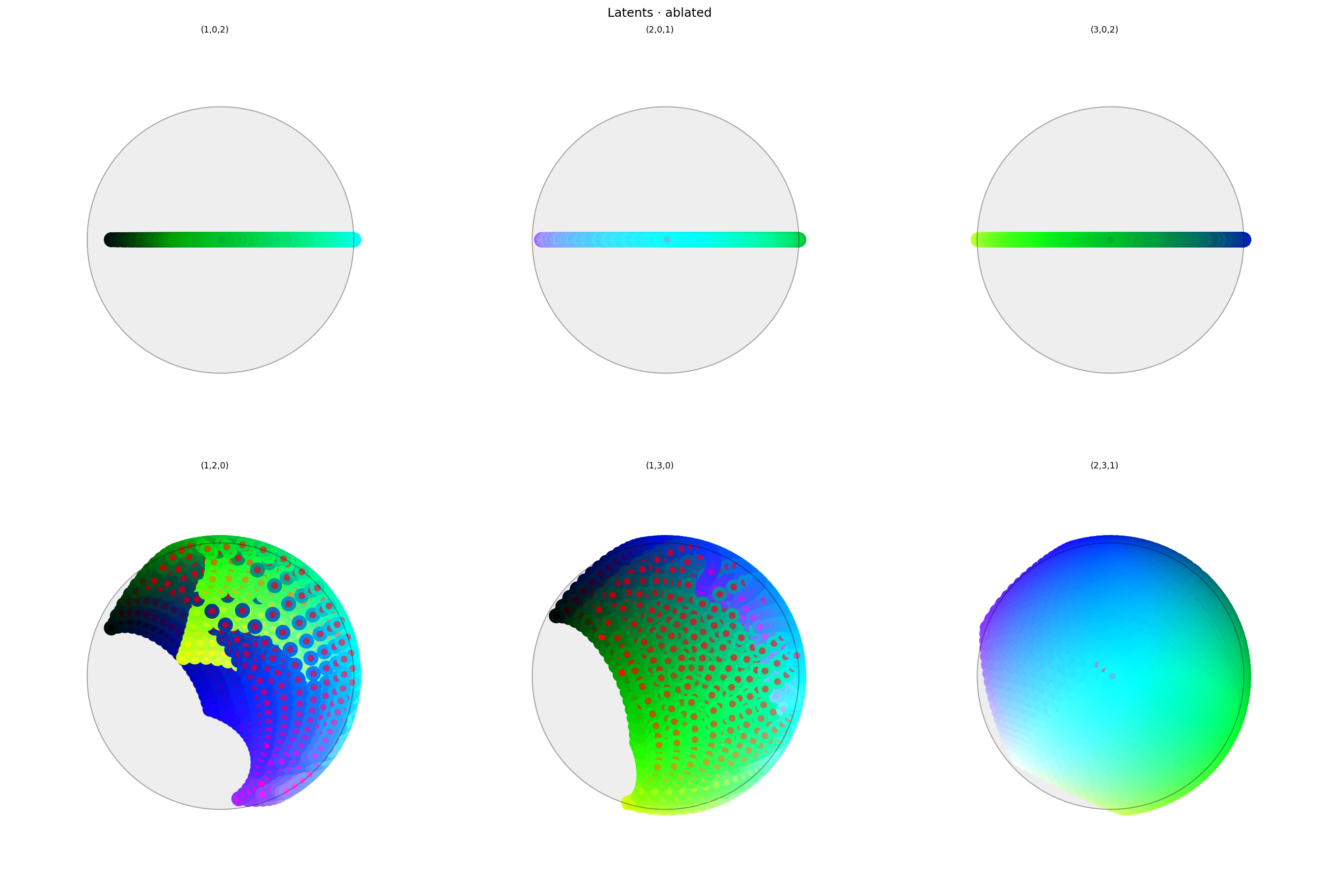
The first dimension has clearly been ablated: there are no points in it at all. But from these plots it's not clear why colors other than red have been so heavily perturbed.