Experiment 2.5: Only one anchor
In earlier experiments like Ex 2.4, we regularized the latent space to look like the color wheel, because it makes it easy to interpret the dynamics of the system. To produce the wheel-like shape with vibrant hues around the rim, those colors were regularized to be planar in the first two dimensions. In effect, the set of vibrant hues were "anchored" to a subspace. But since we're only intervening on one concept (red), the color wheel is unnecessary: it should be possible to get just as good results by only anchoring red, even if the latent space won't be as pretty.
Hypothesis
If we remove the planarity regularizer, the model should perform as well or better than previous models, and the interventions should be at least as precise. We should be able to see that clearly by plotting reconstruction loss vs. hue.
We do not expect to be able to interpret the latent space as clearly as we could in earlier experiments. Here's what we expect to see:
- Red should be in the same place: $(1,0,0,0)$
- Points should be evenly spaced
- Globally it should still look roughly spherical
- Apart from red, vibrant hues will not be constrained to the $(0,1)$ plane — so there will be no "hue" subspace, and no visual color wheel.
from __future__ import annotations

nbid = '2.5'  # ID for tagging assets
nbname = 'Only red'
experiment_name = f'Ex {nbid}: {nbname}'
project = 'ex-preppy'
# Basic setup: Logging, Experiment (Modal)
import logging

import modal

from infra.requirements import freeze, project_packages
from mini.experiment import Experiment
from utils.logging import SimpleLoggingConfig

logging_config = (
    SimpleLoggingConfig()
    .info('notebook', 'utils', 'mini', 'ex_color')
    .error('matplotlib.axes')  # Silence warnings about set_aspect
)
logging_config.apply()

# This is the logger for this notebook
log = logging.getLogger(f'notebook.{nbid}')

run = Experiment(experiment_name, project=project)
run.image = modal.Image.debian_slim().pip_install(*freeze(all=True)).add_local_python_source(*project_packages())
run.before_each(logging_config.apply)
None  # prevent auto-display of this cell
Regularizers
Like Ex 2.4:
- Anchor: pins
redto $(1,0,0,0)$ - Separate: angular repulsion to reduce global clumping (applied within each batch)
- Unitarity: pulls all embeddings to the surface of the unit hypersphere, i.e. it makes the embedding vectors have unit length.
But unlike 2.4:
- Planarity: has been removed.
import torch

from mini.temporal.dopesheet import Dopesheet
from ex_color.loss import Anchor, Separate, Unitarity, RegularizerConfig

from ex_color.training import TrainingModule

RED = (1, 0, 0, 0)

ALL_REGULARIZERS = [
    RegularizerConfig(
        name='reg-unit',
        compute_loss_term=Unitarity(),
        label_affinities=None,
        layer_affinities=['encoder'],
    ),
    RegularizerConfig(
        name='reg-anchor',
        compute_loss_term=Anchor(torch.tensor(RED, dtype=torch.float32)),
        label_affinities={'red': 1.0},
        layer_affinities=['bottleneck'],
    ),
    RegularizerConfig(
        name='reg-separate',
        compute_loss_term=Separate(power=100.0, shift=True),
        label_affinities=None,
        layer_affinities=['bottleneck'],
    ),
]
from functools import partial
from torch import Tensor
from torch.utils.data import DataLoader, TensorDataset, WeightedRandomSampler
import numpy as np

from ex_color.data.color_cube import ColorCube
from ex_color.data.cube_sampler import vibrancy
from ex_color.data.cyclic import arange_cyclic
from ex_color.labelling import collate_with_generated_labels


def prep_data() -> tuple[DataLoader, Tensor]:
    """
    Prepare data for training.

    Returns: (train, val)
    """
    hsv_cube = ColorCube.from_hsv(
        h=arange_cyclic(step_size=10 / 360),
        s=np.linspace(0, 1, 10),
        v=np.linspace(0, 1, 10),
    )
    hsv_tensor = torch.tensor(hsv_cube.rgb_grid.reshape(-1, 3), dtype=torch.float32)
    vibrancy_tensor = torch.tensor(vibrancy(hsv_cube).flatten(), dtype=torch.float32)
    hsv_dataset = TensorDataset(hsv_tensor, vibrancy_tensor)

    labeller = partial(
        collate_with_generated_labels,
        soft=False,  # Use binary labels (stochastic) to simulate the labelling of internet text
        red=0.5,
        vibrant=0.5,
    )
    # Desaturated and dark colors are over-represented in the cube, so we use a weighted sampler to balance them out
    hsv_loader = DataLoader(
        hsv_dataset,
        batch_size=64,
        num_workers=2,
        sampler=WeightedRandomSampler(
            weights=hsv_cube.bias.flatten().tolist(),
            num_samples=len(hsv_dataset),
            replacement=True,
        ),
        collate_fn=labeller,
    )

    rgb_cube = ColorCube.from_rgb(
        r=np.linspace(0, 1, 8),
        g=np.linspace(0, 1, 8),
        b=np.linspace(0, 1, 8),
    )
    rgb_tensor = torch.tensor(rgb_cube.rgb_grid.reshape(-1, 3), dtype=torch.float32)
    return hsv_loader, rgb_tensor
import wandb
from ex_color.inference import InferenceModule
from ex_color.intervention.intervention import InterventionConfig
from ex_color.model import CNColorMLP


# @run.thither(env={'WANDB_API_KEY': wandb.Api().api_key})
async def train(
    dopesheet: Dopesheet,
    regularizers: list[RegularizerConfig],
) -> CNColorMLP:
    """Train the model with the given dopesheet and variant."""
    import lightning as L
    from lightning.pytorch.loggers import WandbLogger

    from ex_color.seed import set_deterministic_mode

    from utils.progress.lightning import LightningProgress

    log.info(f'Training with: {[r.name for r in regularizers]}')

    seed = 0
    set_deterministic_mode(seed)

    hsv_loader, _ = prep_data()

    model = CNColorMLP(4)
    total_params = sum(p.numel() for p in model.parameters() if p.requires_grad)
    log.debug(f'Model initialized with {total_params:,} trainable parameters.')

    training_module = TrainingModule(model, dopesheet, torch.nn.MSELoss(), regularizers)

    logger = WandbLogger(experiment_name, project=project)

    trainer = L.Trainer(
        max_steps=len(dopesheet),
        callbacks=[
            LightningProgress(),
        ],
        enable_checkpointing=False,
        enable_model_summary=False,
        # enable_progress_bar=True,
        logger=logger,
    )

    print(f'max_steps: {len(dopesheet)}, hsv_loader length: {len(hsv_loader)}')

    # Train the model
    try:
        trainer.fit(training_module, hsv_loader)
    finally:
        wandb.finish()
    # This is only a small model, so it's OK to return it rather than storing and loading a checkpoint remotely
    return model


async with run():
    model = await train(Dopesheet.from_csv(f'./ex-{nbid}-dopesheet.csv'), ALL_REGULARIZERS)
I 4.8 no.2.5: Training with: ['reg-unit', 'reg-anchor', 'reg-separate']
INFO: Seed set to 0
I 4.8 li.fa.ut.se:Seed set to 0
I 4.8 ex.se:   PyTorch set to deterministic mode
INFO: GPU available: False, used: False
I 4.8 li.py.ut.ra:GPU available: False, used: False
INFO: TPU available: False, using: 0 TPU cores
I 4.8 li.py.ut.ra:TPU available: False, using: 0 TPU cores
INFO: HPU available: False, using: 0 HPUs
I 4.8 li.py.ut.ra:HPU available: False, using: 0 HPUs
max_steps: 3001, hsv_loader length: 57
wandb: Currently logged in as: z0r to https://api.wandb.ai. Use `wandb login --relogin` to force relogin
./wandb/run-20250905_064141-imud1l1j
Starting phase: Train
INFO: `Trainer.fit` stopped: `max_steps=3001` reached.
I 27.4 li.py.ut.ra:`Trainer.fit` stopped: `max_steps=3001` reached.
Run history:
| epoch | ▁▁▁▂▂▂▂▂▂▃▃▃▃▃▄▄▄▄▄▄▅▅▅▅▅▅▆▆▆▆▆▆▇▇▇▇████ |
| train_loss | █▄▄▆▃▂▄▃▂▂▂▂▃▂▂▂▂▂▂▂▂▂▂▂▂▂▁▁▁▂▁▁▁▁▁▁▁▁▁▁ |
| train_recon | █▂▂▂▂▁▁▁▁▁▁▁▁▁▁▁▁▁▁▂▁▁▁▁▁▁▁▁▁▁▁▁▁▁▁▁▁▁▁▁ |
| train_reg-anchor | ▁▁█▁▁▁▁▁▁▁▂▁▁▁▁▁▁▁▁▁▁▁▁▁▁▁▁▁▁▁▂▁▁▁▁▁▁▁▁▁ |
| train_reg-separate | █▇▆▆▅▇▅▅▃▃▄▂▆▄▃▃▂▁▃▂▄▁▂▄▃▂▃▁▃▃▃▂▄▁▃▃▂▂▂▄ |
| train_reg-unit | █▆▄▂▂▁▁▁▁▁▁▁▁▁▁▁▁▁▁▁▁▁▁▁▁▁▁▁▁▁▁▁▁▁▁▁▁▁▁▁ |
| trainer/global_step | ▁▁▁▂▂▂▃▃▃▃▃▃▄▄▄▄▄▅▅▅▅▅▅▅▅▆▆▆▆▆▆▇▇▇▇▇████ |
Run summary:
| epoch | 52 |
| train_loss | 3e-05 |
| train_recon | 3e-05 |
| train_reg-anchor | 0 |
| train_reg-separate | 0.39431 |
| train_reg-unit | 0.00959 |
| trainer/global_step | 2999 |
View project at: https://wandb.ai/z0r/ex-color-transformer
Synced 5 W&B file(s), 0 media file(s), 0 artifact file(s) and 0 other file(s)
./wandb/run-20250905_064141-imud1l1j/logs
The charts and loss values from training look much the same as last time.
- Roughly the same shape overall
- All loss values roughly the same
# @run.thither
async def infer(
    model: CNColorMLP,
    interventions: list[InterventionConfig],
    test_data: Tensor,
) -> Tensor:
    """Run inference with the given model and interventions."""
    import lightning as L

    inference_module = InferenceModule(model, interventions)
    trainer = L.Trainer(
        enable_checkpointing=False,
        enable_model_summary=False,
        enable_progress_bar=True,
    )
    reconstructed_colors_batches = trainer.predict(
        inference_module,
        DataLoader(
            TensorDataset(test_data.reshape((-1, 3))),
            batch_size=64,
            collate_fn=lambda batch: torch.stack([row[0] for row in batch], 0),
        ),
    )
    assert reconstructed_colors_batches is not None
    # Flatten the list of batches to a single list of tensors
    reconstructed_colors = [item for batch in reconstructed_colors_batches for item in batch]
    # Reshape to match input
    return torch.cat(reconstructed_colors).reshape(test_data.shape)
Let's see how well the model reconstructs colors without any interventions.
from IPython.display import clear_output

from utils.nb import displayer_mpl
from ex_color.vis import plot_colors


hsv_cube = ColorCube.from_hsv(
    h=arange_cyclic(step_size=1 / 24),
    s=np.linspace(0, 1, 4),
    v=np.linspace(0, 1, 8),
).permute('svh')
x_hsv = torch.tensor(hsv_cube.rgb_grid, dtype=torch.float32)

hd_hsv_cube = ColorCube.from_hsv(
    h=arange_cyclic(step_size=1 / 240),
    s=np.linspace(0, 1, 48),
    v=np.linspace(0, 1, 48),
)
hd_x_hsv = torch.tensor(hd_hsv_cube.rgb_grid, dtype=torch.float32)

rgb_cube = ColorCube.from_rgb(
    r=np.linspace(0, 1, 20),
    g=np.linspace(0, 1, 20),
    b=np.linspace(0, 1, 20),
)
x_rgb = torch.tensor(rgb_cube.rgb_grid, dtype=torch.float32)

with displayer_mpl(
    f'large-assets/ex-{nbid}-true-colors.png',
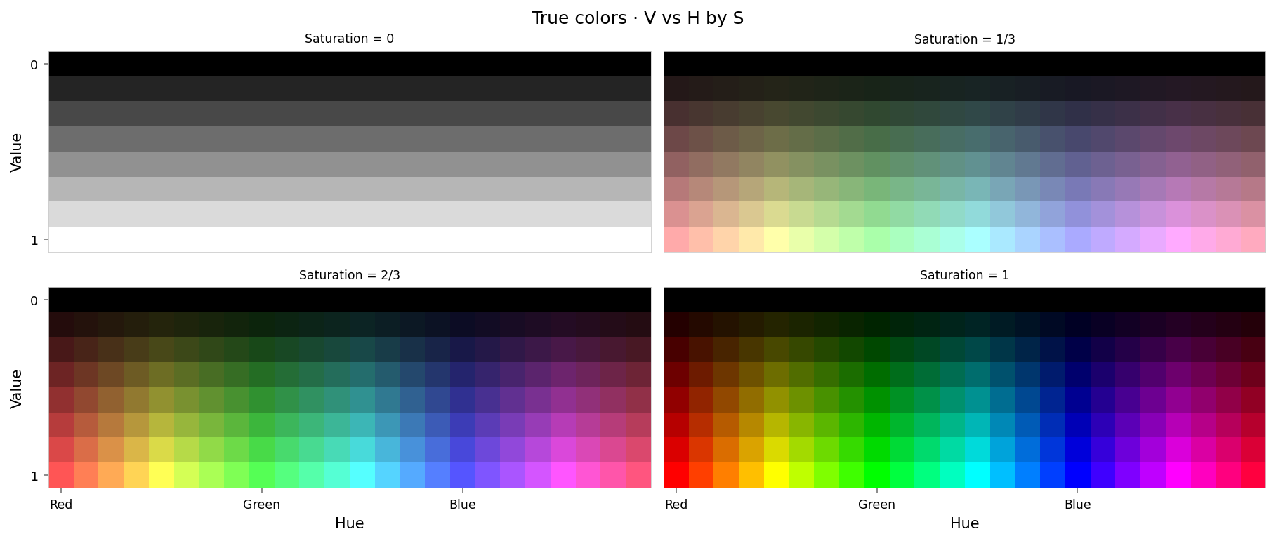
    alt_text="""Plot showing four slices of the HSV cube, titled "{title}". Each slice has constant saturation, but varies in value (brightness) from top to bottom, and in hue from left to right. The first slice shows a grayscale gradient from black to white; the last shows the fully-saturated color spectrum.""",
) as show:
    show(lambda: plot_colors(hsv_cube, title='True colors', colors=x_hsv.numpy()))
from IPython.display import clear_output
from torch.nn import functional as F

from ex_color.vis import plot_colors, plot_cube_series


interventions = []
y_hsv = await infer(model, interventions, x_hsv)
hd_y_hsv = await infer(model, interventions, hd_x_hsv)
clear_output()

with displayer_mpl(
    f'large-assets/ex-{nbid}-pred-colors-no-intervention.png',
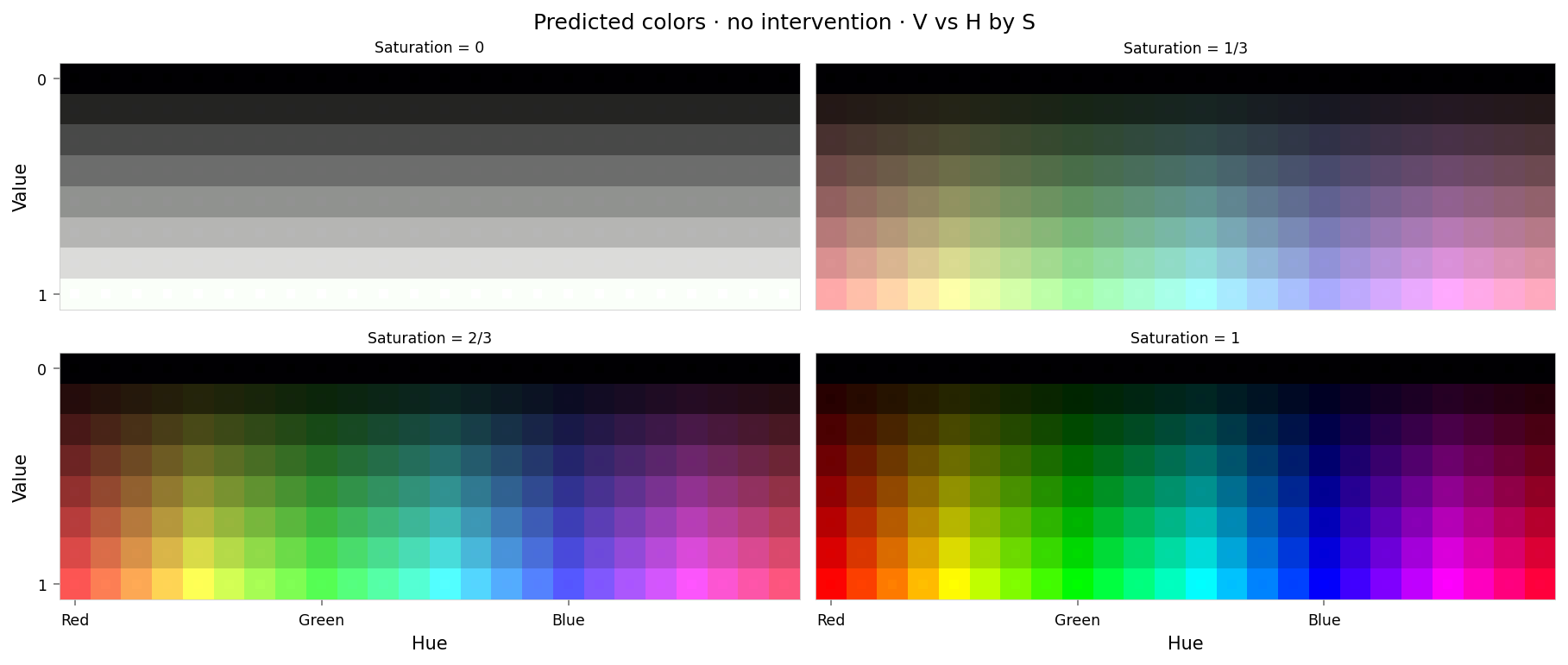
    alt_text="""Plot showing four slices of the HSV cube, titled "{title}". Nominally, each slice has constant saturation, but varies in value (brightness) from top to bottom, and in hue from left to right. Each color value is represented as a square patch of that color. The outer portion of the patches shows the color as reconstructed by the model; the inner portion shows the true (input) color. The reconstructed and true colors agree fairly well, but some slight differences are visible; for example, "white" is slightly gray, and many of the fully-saturated colors are less saturated than they should be.""",
) as show:
    show(
        lambda: plot_colors(
            hsv_cube,
            title='Predicted colors · no intervention',
            colors=y_hsv.numpy(),
            colors_compare=x_hsv.numpy(),
        )
    )

per_color_loss = F.mse_loss(hd_y_hsv, hd_x_hsv, reduction='none').mean(dim=-1)
loss_cube = hd_hsv_cube.assign('MSE', per_color_loss.numpy().reshape(hd_hsv_cube.shape))
max_loss = per_color_loss.max().item()
median_loss = per_color_loss.median().item()
with displayer_mpl(
    f'large-assets/ex-{nbid}-loss-colors-no-intervention.png',
    alt_text=f"""Line chart showing loss per color, titled "{{title}}". Y-axis: mean square error, ranging from zero to {max_loss:.2g}. X-axis: hue. The range of loss values is small, but there are two notable peaks at all primary and secondary colors (red, yellow, green, etc.).""",
) as show:
    show(
        lambda: plot_cube_series(
            loss_cube.permute('hsv')[:, -1:, :: (loss_cube.shape[2] // -5)],
            loss_cube.permute('svh')[:, -1:, :: -(loss_cube.shape[0] // -3)],
            loss_cube.permute('vsh')[:, -1:, :: -(loss_cube.shape[0] // -3)],
            title='Reconstruction error · no intervention',
            var='MSE',
            figsize=(12, 3),
        )
    )
print(f'Max loss: {max_loss:.2g}')
print(f'Median MSE: {median_loss:.2g}')

Max loss: 0.00028
Median MSE: 1.4e-05
That looks similar to 2.4 but with an order of magnitude lower max loss.
# Capture encoder activations (latents) without interventions
import torch
import numpy as np

from ex_color.inference import InferenceModule


# Build a tiny helper that runs predict while capturing latents from 'encoder'
async def infer_with_latent_capture(
    model: CNColorMLP, interventions: list[InterventionConfig], test_data: Tensor, layer_name: str = 'bottleneck'
) -> tuple[Tensor, Tensor]:
    module = InferenceModule(model, interventions, capture_layers=[layer_name])
    import lightning as L

    trainer = L.Trainer(enable_checkpointing=False, enable_model_summary=False, enable_progress_bar=False)
    batches = trainer.predict(
        module,
        DataLoader(
            TensorDataset(test_data.reshape((-1, 3))),
            batch_size=64,
            collate_fn=lambda batch: torch.stack([row[0] for row in batch], 0),
        ),
    )
    assert batches is not None
    preds = [item for batch in batches for item in batch]
    y = torch.cat(preds).reshape(test_data.shape)
    # Read captured activations as a flat [N, D] tensor
    latents = module.read_captured(layer_name)
    return y, latents
from IPython.display import clear_output

from ex_color.vis import plot_latent_grid_3d

y_rgb, h_rgb = await infer_with_latent_capture(model, [], x_rgb, 'bottleneck')
clear_output()

with displayer_mpl(
    f'large-assets/ex-{nbid}-latents-no-intervention.png',
    alt_text="""Three spherical plots, titled "{title}". Each plot shows a view of vibrant collection of colored circles or balls scattered over the surface of a sphere. The points look structured, but not in any clear way, except that similar colors are close to each other. Red is at the top of the first plot, and in the center of the other two.""",
) as show:
    show(
        lambda theme: plot_latent_grid_3d(
            h_rgb,
            y_rgb,
            x_rgb,
            title='Latents · no intervention',
            dims=[(1, 0, 2), (1, 2, 0), (1, 3, 0)],
            dot_radius=10,
            theme=theme,
        )
    )
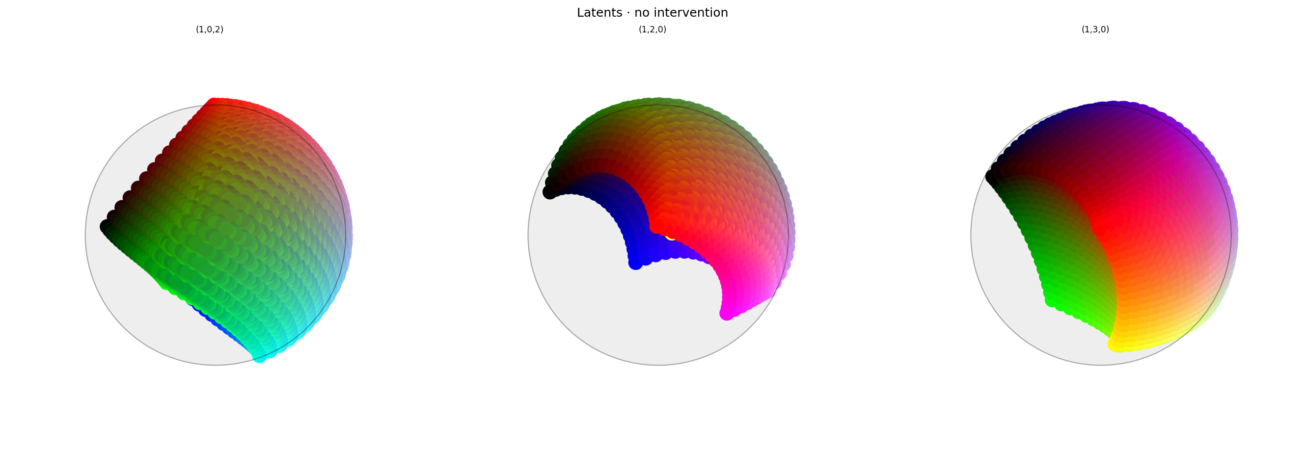
As expected: without any intervention, the latent space looks ball-shaped but there's no visible color wheel. Vibrant hues are positioned arbitrarily, but red is still at the $(1,0,0,0)$ anchor point.
Suppression
Now that we have our model, let's try suppressing red. We'll use the Suppression function developed in Ex 2.1.
from math import cos, pi

import torch

from ex_color.intervention import BoundedFalloff, InterventionConfig, Suppression
from ex_color.vis import plot_colors, plot_cube_series


suppression = Suppression(
    torch.tensor(RED, dtype=torch.float32),  # Constant!
    BoundedFalloff(
        0,  # within 60°
        1,  # completely squash fully-aligned vectors
        2,  # soft rim, sharp hub
    ),
)

interventions = [InterventionConfig(suppression, ['bottleneck'])]
y_hsv = await infer(model, interventions, x_hsv)
hd_y_hsv = await infer(model, interventions, hd_x_hsv)
clear_output()

with displayer_mpl(
    f'large-assets/ex-{nbid}-pred-colors-suppression.png',
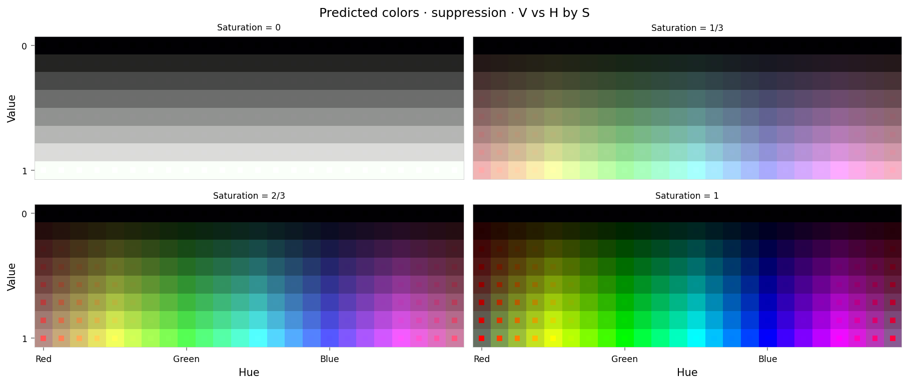
    alt_text="""Plot showing four slices of the HSV cube, titled "{title}". Nominally, each slice has constant saturation, but varies in value (brightness) from top to bottom, and in hue from left to right. Each color value is represented as a square patch of that color. The outer portion of the patches shows the color as reconstructed by the model; the inner portion shows the true (input) color. The reconstructed and true colors agree fairly well, but "red" and nearby colors are clearly different: red itself appears as middle-gray, and the surrounding colors up to orange and pink look washed out. "Red-orange" actually appears to be green, moreso even than yellow (which is geometrically closer to green).""",
) as show:
    show(
        lambda: plot_colors(
            hsv_cube,
            title='Predicted colors · suppression',
            colors=y_hsv.numpy(),
            colors_compare=x_hsv.numpy(),
        )
    )

per_color_loss = F.mse_loss(hd_y_hsv, hd_x_hsv, reduction='none').mean(dim=-1)
loss_cube = hd_hsv_cube.assign('MSE', per_color_loss.numpy().reshape(hd_hsv_cube.shape))
max_loss = per_color_loss.max().item()
median_loss = per_color_loss.median().item()
with displayer_mpl(
    f'large-assets/ex-{nbid}-loss-colors-suppression.png',
    alt_text=f"""Line chart showing loss per color, titled "{{title}}". Y-axis: mean square error, ranging from zero to {max_loss:.2g}. X-axis: hue. There is a significant peak at red at either end of the X-axis, gradually sloping down to lower loss values near yellow and pink. Two very small peaks are at green and blue (apparently around 1% of the height of the peaks at red).""",
) as show:
    show(
        lambda: plot_cube_series(
            loss_cube.permute('hsv')[:, -1:, :: (loss_cube.shape[2] // -5)],
            loss_cube.permute('svh')[:, -1:, :: -(loss_cube.shape[0] // -6)],
            loss_cube.permute('vsh')[:, -1:, :: -(loss_cube.shape[0] // -6)],
            title='Reconstruction error · suppression',
            var='MSE',
            figsize=(12, 3),
        )
    )
print(f'Max loss: {max_loss:.2g}')
print(f'Median MSE: {median_loss:.2g}')

Max loss: 0.23
Median MSE: 2.2e-05
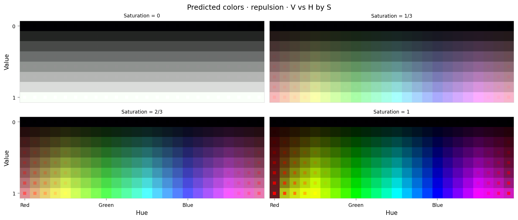
These plots are somewhat interesting: visually, the reconstructed colors diverge to a similar amount as in the previous experiment but in a different direction. Previously red moved to a kind of dull, dark red; here it seems to have become more green or gray.
Looking at loss vs. hue, the intervention seems to have a similar effect on yellow and pink, while the max loss (at red) is higher. The curves have become a little messier, crossing over each other more than in 2.4. This might suggest that the latent space is a little less smooth/regular.
from IPython.display import clear_output

from ex_color.vis import plot_latent_grid_3d, ConicalAnnotation

# Capture latents with suppression
y_rgb, h_rgb = await infer_with_latent_capture(model, interventions, x_rgb, 'bottleneck')
clear_output()

with displayer_mpl(
    f'large-assets/ex-{nbid}-latents-suppression.png',
    alt_text="""Three spherical plots, titled "{title}". Each plot shows a view of vibrant collection of colored circles or balls scattered over the surface of a sphere. The points look structured, but not in any clear way, except that similar colors are close to each other. The first plot has a conspicuously empty space at the top. The center of the middle plot looks messy.""",
) as show:
    show(
        lambda theme: plot_latent_grid_3d(
            h_rgb,
            y_rgb,
            x_rgb,
            title='Latents · suppression',
            dims=[(1, 0, 2), (1, 2, 0), (1, 3, 0)],
            dot_radius=10,
            theme=theme,
            annotations=[
                ConicalAnnotation(
                    RED,
                    2 * (np.pi / 2 - suppression.falloff.a),  # type: ignore
                    color=theme.val('black', dark='#fffa'),
                    linewidth=theme.val(0.5, dark=1),
                    dashes=theme.val((8, 8), dark=(4, 4)),
                    gapcolor=theme.val('#fff4', dark='#0004'),
                ),
            ],
        )
    )
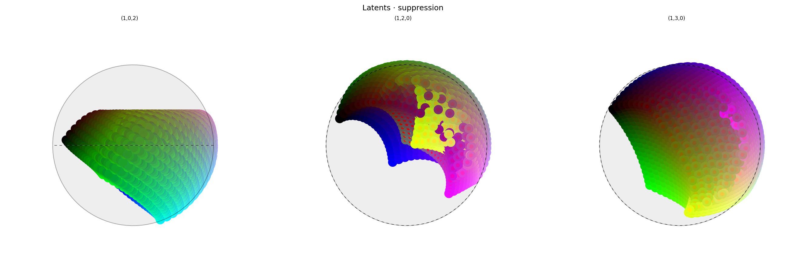
As expected, the intervention has had the same squashing effect on the latent space, pushing red into the middle of the sphere. The intervention is just as clear in the first view (in which y is the axis of intervention). The other plots (in which z is the axis of intervention) are harder to interpret because of the placement of colors like white, but the ring at the edge of the intervention is still visible.
from math import cos, pi

import torch

from ex_color.intervention import FastBezierMapper, InterventionConfig, Repulsion
from ex_color.vis import plot_colors, plot_cube_series

repulsion = Repulsion(
    torch.tensor([1, 0, 0, 0], dtype=torch.float32),  # Constant!
    FastBezierMapper(
        0,  # Constrain effect to within 60° cone
        cos(pi / 3),  # Create 30° hole (negative cone) around concept vector
    ),
)


interventions = [InterventionConfig(repulsion, ['bottleneck'])]
y_hsv = await infer(model, interventions, x_hsv)
hd_y_hsv = await infer(model, interventions, hd_x_hsv)
clear_output()

with displayer_mpl(
    f'large-assets/ex-{nbid}-pred-colors-repulsion.png',
    alt_text="""Plot showing four slices of the HSV cube, titled "{title}". Nominally, each slice has constant saturation, but varies in value (brightness) from top to bottom, and in hue from left to right. Each color value is represented as a square patch of that color. The outer portion of the patches shows the color as reconstructed by the model; the inner portion shows the true (input) color. The reconstructed and true colors agree fairly well, but "red" and nearby colors are clearly different, and different again from how the suppression intervention looked: "red" itself appears as pink or hot pink, and the surrounding colors up to orange and pink look shifted. "Red-orange" actually appears to be fully-saturated yellow. Overall the effect is as though the nearby colors have bled into the neighborhood of red.""",
) as show:
    show(
        lambda: plot_colors(
            hsv_cube,
            title='Predicted colors · repulsion',
            colors=y_hsv.numpy(),
            colors_compare=x_hsv.numpy(),
        )
    )


per_color_loss = F.mse_loss(hd_y_hsv, hd_x_hsv, reduction='none').mean(dim=-1)
loss_cube = hd_hsv_cube.assign('MSE', per_color_loss.numpy().reshape(hd_hsv_cube.shape))
max_loss = per_color_loss.max().item()
median_loss = per_color_loss.median().item()
with displayer_mpl(
    f'large-assets/ex-{nbid}-loss-colors-repulsion.png',
    alt_text=f"""Line chart showing loss per color, titled "{{title}}". Y-axis: mean square error, ranging from zero to {max_loss:.2g}. X-axis: hue. There is a significant peak at red at either end of the X-axis, gradually sloping down to lower loss values near yellow and pink. Two very small peaks are at green and blue (apparently less than 1% of the height of the peaks at red).""",
) as show:
    show(
        lambda: plot_cube_series(
            loss_cube.permute('hsv')[:, -1:, :: (loss_cube.shape[2] // -5)],
            loss_cube.permute('svh')[:, -1:, :: -(loss_cube.shape[0] // -6)],
            loss_cube.permute('vsh')[:, -1:, :: -(loss_cube.shape[0] // -6)],
            title='Reconstruction error · repulsion',
            var='MSE',
            figsize=(12, 3),
        )
    )
print(f'Max loss: {max_loss:.2g}')
print(f'Median MSE: {median_loss:.2g}')

Max loss: 0.14
Median MSE: 2.7e-05
These plots look similar to those from 2.4, but again they show a higher maximum loss at red and more overlap of the various curves.
from IPython.display import clear_output

from ex_color.vis import plot_latent_grid_3d, ConicalAnnotation

# Capture latents with repulsion
y_rgb, h_rgb = await infer_with_latent_capture(model, interventions, x_rgb, 'bottleneck')
clear_output()

with displayer_mpl(
    f'large-assets/ex-{nbid}-latents-repulsion.png',
    alt_text="""Three spherical plots, titled "{title}". Each plot shows a view of vibrant collection of colored circles or balls scattered over the surface of a sphere. The points look structured, but not in any clear way, except that similar colors are close to each other. The first plot has a conspicuously empty space at the top. The center of the middle plot looks messy, but it shows a clear ring of points with red dots in the middle, showing where red colors have been repelled to.""",
) as show:
    show(
        lambda theme: plot_latent_grid_3d(
            h_rgb,
            y_rgb,
            x_rgb,
            title='Latents · repulsion',
            dims=[(1, 0, 2), (1, 2, 0), (1, 3, 0)],
            dot_radius=10,
            theme=theme,
            annotations=[
                ConicalAnnotation(
                    RED,
                    2 * (np.pi / 2 - repulsion.mapper.a),  # type: ignore
                    color=theme.val('black', dark='#fffa'),
                    linewidth=theme.val(0.5, dark=1),
                    dashes=theme.val((8, 8), dark=(4, 4)),
                    gapcolor=theme.val('#fff4', dark='#0004'),
                ),
                ConicalAnnotation(
                    RED,
                    2 * (np.pi / 2 - repulsion.mapper.b),  # type: ignore
                    color=theme.val('black', dark='#fffa'),
                    linewidth=theme.val(0.5, dark=1),
                ),
            ],
        )
    )
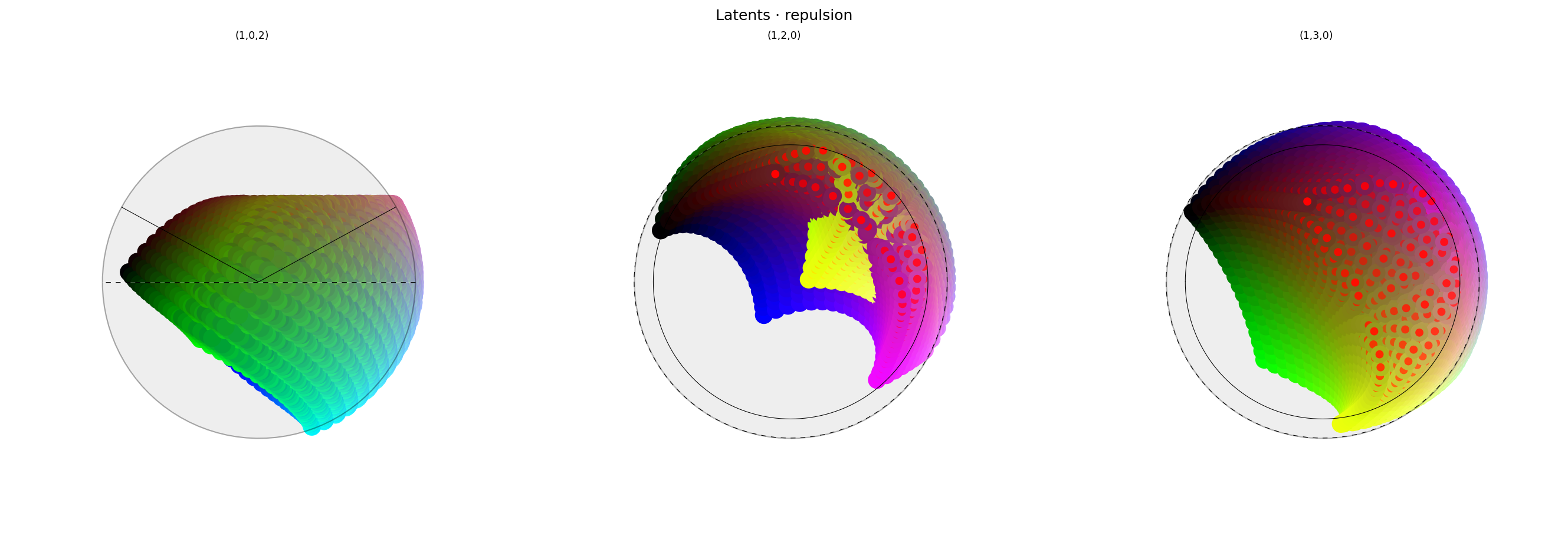
And again, the effect of the intervention is clear in the plot on the left, in which y is the axis of intervention. The other plots show that red colors have been pushed to the edge of the cone — the ring is clearly visible — but it's hard to interpret where they have been pushed to.
The spacing of the points is fairly regular, but visually less so than 2.4. That's a little surprising: having fewer constraints should have made it easier to satisfy the remaining regularizers. Indeed the measured loss for the separation term is lower; perhaps that just means it was able to push points further from each other because it was able to make use of more of the surface of the hypersphere. The planarity term previously constrained all points to be in a hemi-hypersphere. The network would have had to balance the compactness encouraged by planarity with the sparseness encouraged by the separation term. Alternatively this could have happened by chance: the difference is small, and we only ran it with one seed.
Conclusion
Hypothesis: partially confirmed. Without the planarity regularization term:
- The network reached a lower max reconstruction loss
- Vibrant hues other than red were positioned arbitrarily on the surface of the hypersphere, so no color wheel was visible
- Red was successfully positioned at the anchor point.
However, the interventions weren't quite as precise as before. Perhaps they could be better with some hyperparameter tuning (we didn't tune them at all).