Experiment 2.10: Delete only red without "desaturated" label

In Ex 2.9 we succeed in deleting red without deleting cyan or other colors, with precision similar to an intervention with a cosine falloff. In that experiment, we used a subspace regularizer to attract desaturated colors to the last three dimensions. Let's see if we can get similar results without that label. We'll also try removing the unitarity regularizer to verify that it's still needed.

Hypothesis

If we weakly repel all embeddings from the anchor dimension, then we will be able to delete red without also deleting other colors. We should see error vs. color curves similar to those achieved in 2.9.

from __future__ import annotations

nbid = '2.10'  # ID for tagging assets
nbname = 'Ablate red (only), 5D, fewer labels'
experiment_name = f'Ex {nbid}: {nbname}'
project = 'ex-preppy'

# Basic setup: Logging, Experiment (Modal)
import logging

import modal

from infra.requirements import freeze, project_packages
from mini.experiment import Experiment
from utils.logging import SimpleLoggingConfig

logging_config = (
    SimpleLoggingConfig()
    .info('notebook', 'utils', 'mini', 'ex_color')
    .error('matplotlib.axes')  # Silence warnings about set_aspect
)
logging_config.apply()

# This is the logger for this notebook
log = logging.getLogger(f'notebook.{nbid}')

run = Experiment(experiment_name, project=project)
run.image = modal.Image.debian_slim().pip_install(*freeze(all=True)).add_local_python_source(*project_packages())
run.before_each(logging_config.apply)
None  # prevent auto-display of this cell

Model parameters

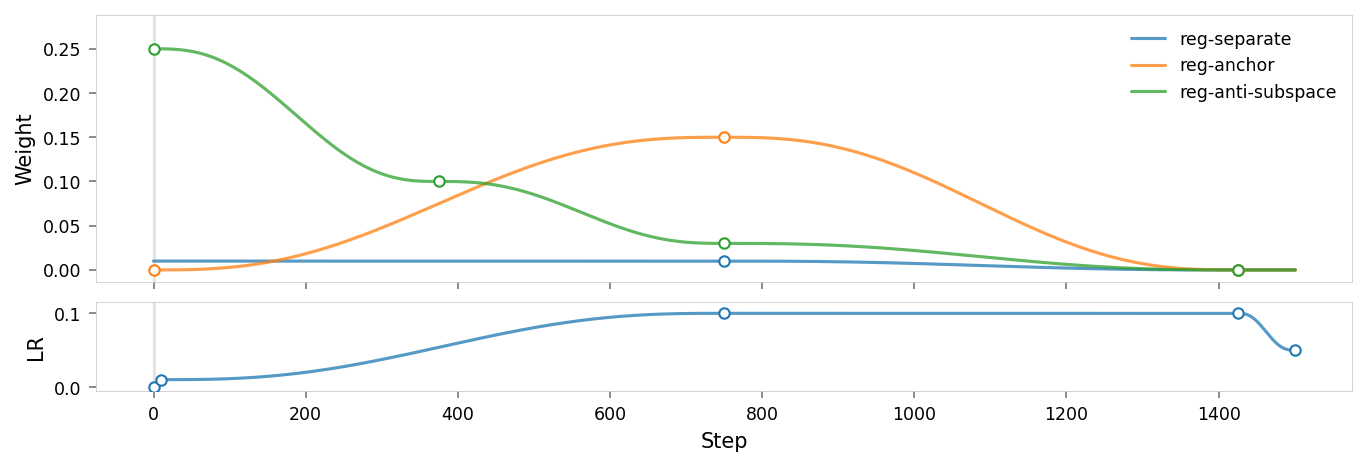
Like Ex 2.9, we use the following regularizers:

• Anchor: pins red to $(1,0,0,0,0)$ (5D)
• AxisAlignedSubspace: repels everything from dimension $1$ (with varying weight, see schedule)
• Separate: angular repulsion to reduce global clumping (applied within each batch)

Since we're isolating red, we have 5D latent embeddings and two nonlinear activation functions in the encoder and decoder, to allow the latent space to be warped more.

But unlike 2.9:

• Anti-anchor: has been removed, relying on anti-subspace to keep other concepts clear of the dimension to be ablated.
• Unitarity: is present in this list, but we'll do a run without it too.

import torch

from ex_color.loss import AngularAnchor, AxisAlignedSubspace, Separate, RegularizerConfig

from ex_color.training import TrainingModule

K = 5  # bottleneck dimensionality
N = 2  # number of nonlinear layers
RED = (1, 0, 0, 0, 0)

reg_separate = RegularizerConfig(
    name='reg-separate',
    compute_loss_term=Separate(power=100.0, shift=True),
    label_affinities=None,
    layer_affinities=['bottleneck'],
)
reg_anchor = RegularizerConfig(
    name='reg-anchor',
    compute_loss_term=AngularAnchor(torch.tensor(RED, dtype=torch.float32)),
    label_affinities={'red': 1.0},
    layer_affinities=['bottleneck'],
    phase=('train', 'validate'),
)
reg_anti_subspace = RegularizerConfig(
    name='reg-anti-subspace',
    compute_loss_term=AxisAlignedSubspace((0,), invert=True),
    label_affinities=None,
    layer_affinities=['bottleneck'],
)

from typing import cast

import matplotlib.pyplot as plt
from matplotlib.axes import Axes
from IPython.display import display, Markdown

from mini.temporal.dopesheet import Dopesheet
from mini.temporal.timeline import Timeline
from mini.temporal.vis import plot_timeline, realize_timeline, ParamGroup
from utils.nb import displayer_mpl
from utils.plt import Theme

dopesheet = Dopesheet.from_csv(f'./ex-{nbid}-dopesheet.csv')

display(Markdown(f"""## Parameter schedule \n{dopesheet.to_markdown()}"""))


def plot_dopesheet(dopesheet: Dopesheet, theme: Theme):
    timeline = Timeline(dopesheet)
    history_df = realize_timeline(timeline)
    keyframes_df = dopesheet.as_df()

    fig = plt.figure(figsize=(9, 3), constrained_layout=True)
    axs = fig.subplots(2, 1, sharex=True, height_ratios=[3, 1])
    ax1, ax2 = cast(tuple[Axes, ...], axs)

    plot_timeline(
        history_df,
        keyframes_df,
        groups=(ParamGroup(name='', params=[p for p in dopesheet.props if p not in {'lr'}]),),
        theme=theme,
        ax=ax1,
        show_phase_labels=False,
    )
    ax1.set_ylabel('Weight')
    ax1.set_xlabel('')

    plot_timeline(
        history_df,
        keyframes_df,
        groups=(ParamGroup(name='', params=['lr']),),
        theme=theme,
        ax=ax2,
        show_legend=False,
        show_phase_labels=False,
    )
    ax2.set_ylabel('LR')

    # add a little space on the y-axis extents
    ax1.set_ylim(ax1.get_ylim()[0] * 1.1, ax1.get_ylim()[1] * 1.1)
    ax2.set_ylim(ax2.get_ylim()[0] * 1.1, ax2.get_ylim()[1] * 1.1)

    return fig


with displayer_mpl(
    f'large-assets/ex-{nbid}-dopesheet.png',
    alt_text="""Plot showing the parameter schedule for the training run, titled "{title}". The plot has two sections: the upper section shows various regularization weights over time, and the lower section shows the learning rate over time. The x-axis represents training steps.""",
) as show:
    show(lambda theme: plot_dopesheet(dopesheet, theme))

Parameter schedule

STEP	PHASE	ACTION	lr	reg-separate	reg-anchor	reg-anti-subspace
0	Train		1e-08		0	0.25
10			0.01
375						0.1
750			0.1	0.01	0.15	0.03
1425			0.1	0	0	0
1500			0.05

Data

Data is the same as last time: color cubes with values in RGB.

from torch import Tensor
from torch.utils.data import DataLoader, TensorDataset, RandomSampler
import numpy as np

from ex_color.data.color_cube import ColorCube
from ex_color.data.cube_dataset import CubeDataset, redness, stochastic_labels, exact_labels

# from ex_color.data.cube_sampler import vibrancy
from ex_color.data.cyclic import arange_cyclic


def prep_data() -> DataLoader:
    cube = ColorCube.from_rgb(
        r=np.linspace(0, 1, 10),
        g=np.linspace(0, 1, 10),
        b=np.linspace(0, 1, 10),
    )
    # Softly label _red_ - will be stochastically discretized in the dataloader
    cube = cube.assign(
        red=redness(cube['color']) ** 8 * 0.08,
        # vibrant=vibrancy(cube['color']) ** 100 * 0.02,
        # desaturated=(1 - vibrancy(cube['color'])) ** 10 * 0.02,
    )
    dataset = CubeDataset(cube)
    return DataLoader(
        dataset,
        batch_size=64,
        num_workers=4,
        sampler=RandomSampler(dataset, num_samples=len(dataset), replacement=True),
        collate_fn=stochastic_labels,
    )


def prep_val_data() -> DataLoader:
    cube = ColorCube.from_rgb(
        r=np.linspace(0, 1, 4),
        g=np.linspace(0, 1, 4),
        b=np.linspace(0, 1, 4),
    )
    # Exact labels for validation: we only check where the prototypes are located
    cube = cube.assign(
        red=redness(cube['color']) == 1,
        # vibrant=vibrancy(cube['color']) == 1,
    )
    dataset = CubeDataset(cube)
    return DataLoader(
        dataset,
        # batch_size=len(dataset),
        num_workers=2,
        collate_fn=exact_labels,
    )

import numpy as np

from ex_color.data.color_cube import ColorCube
from ex_color.data.cyclic import arange_cyclic

hsv_cube = ColorCube.from_hsv(
    h=arange_cyclic(step_size=1 / 24),
    s=np.linspace(0, 1, 4),
    v=np.linspace(0, 1, 8),
).permute('svh')

hd_hsv_cube = ColorCube.from_hsv(
    h=arange_cyclic(step_size=1 / 240),
    s=np.linspace(0, 1, 48),
    v=np.linspace(0, 1, 48),
)
hd_hsv_cube = hd_hsv_cube[::2, ::2, ::2]

rgb_cube = ColorCube.from_rgb(
    r=np.linspace(0, 1, 20),
    g=np.linspace(0, 1, 20),
    b=np.linspace(0, 1, 20),
)

# with displayer_mpl(
#     f'large-assets/ex-{nbid}-true-colors.png',
#     alt_text="""Plot showing four slices of the HSV cube, titled "{title}". Each slice has constant saturation, but varies in value (brightness) from top to bottom, and in hue from left to right. The first slice shows a grayscale gradient from black to white; the last shows the fully-saturated color spectrum.""",
# ) as show:
#     show(lambda: plot_colors(hsv_cube, title='True colors'))

Training & inference utils

Like in Ex 2.2..2.9, the model is trained with PyTorch Lightning, with regularizers applied as custom hooks.

from tempfile import gettempdir
import wandb
from ex_color.model import CNColorMLP


# @run.thither(env={'WANDB_API_KEY': wandb.Api().api_key})
async def train(
    dopesheet: Dopesheet,
    regularizers: list[RegularizerConfig],
    k_bottleneck: int,
    n_nonlinear: int,
    *,
    seed: int | None = None,
) -> CNColorMLP:
    """Train the model with the given dopesheet and variant."""
    import lightning as L
    from lightning.pytorch.loggers import WandbLogger

    from ex_color.callbacks import LabelProportionCallback
    from ex_color.seed import set_deterministic_mode

    from utils.progress.lightning import LightningProgress

    log.info(f'Training with: {[r.name for r in regularizers]}')

    if seed is not None:
        set_deterministic_mode(seed)

    train_loader = prep_data()
    val_loader = prep_val_data()

    model = CNColorMLP(k_bottleneck, n_nonlinear=n_nonlinear)
    total_params = sum(p.numel() for p in model.parameters() if p.requires_grad)
    log.debug(f'Model initialized with {total_params:,} trainable parameters.')

    training_module = TrainingModule(model, dopesheet, torch.nn.MSELoss(), regularizers)

    logger = WandbLogger(experiment_name, project=project, save_dir=gettempdir())

    trainer = L.Trainer(
        max_steps=len(dopesheet),
        callbacks=[
            LightningProgress(),
            LabelProportionCallback(prefix='labels', get_active_labels=lambda: training_module.active_labels),
        ],
        enable_checkpointing=False,
        enable_model_summary=False,
        # enable_progress_bar=True,
        check_val_every_n_epoch=10,
        logger=logger,
        log_every_n_steps=min(50, len(train_loader)),
    )

    print(f'max_steps: {len(dopesheet)}, train_loader length: {len(train_loader)}')

    # Train the model
    try:
        trainer.fit(training_module, train_loader, val_loader)
    finally:
        wandb.finish()
    # This is only a small model, so it's OK to return it rather than storing and loading a checkpoint remotely
    return model

We wrap the model that we trained above in an InferenceModule. We won't be using its intervention features.

import torch
import numpy as np

from ex_color.inference import InferenceModule


async def infer_with_latent_capture(
    model: CNColorMLP,
    test_data: Tensor,
    layer_name: str = 'bottleneck',
) -> tuple[Tensor, Tensor]:
    module = InferenceModule(model, [], capture_layers=[layer_name])
    import lightning as L

    trainer = L.Trainer(enable_checkpointing=False, enable_model_summary=False, enable_progress_bar=False, logger=False)
    batches = trainer.predict(
        module,
        DataLoader(
            TensorDataset(test_data.reshape((-1, 3))),
            batch_size=64,
            collate_fn=lambda batch: torch.stack([row[0] for row in batch], 0),
        ),
    )
    assert batches is not None
    preds = [item for batch in batches for item in batch]
    y = torch.cat(preds).reshape(test_data.shape)
    # Read captured activations as a flat [N, D] tensor
    latents = module.read_captured(layer_name)
    return y, latents

from torch.nn import functional as F


async def test(model: CNColorMLP, test_data: ColorCube) -> ColorCube:
    x = torch.tensor(test_data.rgb_grid, dtype=torch.float32)
    y, h = await infer_with_latent_capture(model, x, 'bottleneck')
    per_color_loss = F.mse_loss(y, x, reduction='none').mean(dim=-1)
    return test_data.assign(
        recon=y.numpy().reshape((*test_data.shape, -1)),
        MSE=per_color_loss.numpy().reshape((*test_data.shape, -1)),
        latents=h.numpy().reshape((*test_data.shape, -1)),
    )

# # Generate a list of dimensions to visualize
# from itertools import combinations
# [
#     (
#         b,
#         a,
#         (a + 1) % 5 if (a + 1) % 5 not in (a, b) else (a + 2) % 5,
#     )
#     for a, b in combinations((0, 1, 2, 3, 4), 2)
# ]

from typing import Sequence

from ex_color.vis import plot_colors, plot_cube_series, plot_latent_grid_3d_from_cube
from utils.nb import displayer_mpl


def tags_for_file(tags: Sequence[str]) -> str:
    import re

    tags = [re.sub(r'[^a-zA-Z0-9]+', '-', tag.lower()) for tag in tags]
    return '-'.join(tags)


def visualize_reconstructed_cube(data: ColorCube, *, tags: Sequence[str] = ()):
    with displayer_mpl(
        f'large-assets/ex-{nbid}-pred-colors-{tags_for_file(tags)}.png',
        alt_text="""Plot showing four slices of the HSV cube, titled "{title}". Nominally, each slice has constant saturation, but varies in value (brightness) from top to bottom, and in hue from left to right. Each color value is represented as a square patch of that color. The outer portion of the patches shows the color as reconstructed by the model; the inner portion shows the true (input) color.""",
    ) as show:
        show(
            lambda: plot_colors(
                data,
                title=f'Predicted colors · {" · ".join(tags)}',
                colors='recon',
                colors_compare='color',
            )
        )


def visualize_reconstruction_loss(data: ColorCube, *, tags: Sequence[str] = ()):
    max_loss = np.max(data['MSE'])
    median_loss = np.median(data['MSE'])
    with displayer_mpl(
        f'large-assets/ex-{nbid}-loss-colors-{tags_for_file(tags)}.png',
        alt_text=f"""Line chart showing loss per color, titled "{{title}}". Y-axis: mean square error, ranging from zero to {max_loss:.2g}. X-axis: hue.""",
    ) as show:
        show(
            lambda: plot_cube_series(
                data.permute('hsv')[:, -1:, :: (data.shape[2] // -5)],
                data.permute('svh')[:, -1:, :: -(data.shape[0] // -3)],
                data.permute('vsh')[:, -1:, :: -(data.shape[0] // -3)],
                title=f'Reconstruction error · {" · ".join(tags)}',
                var='MSE',
                figsize=(12, 3),
            )
        )
    print(f'Max loss: {max_loss:.2g}')
    print(f'Median MSE: {median_loss:.2g}')


def visualize_latent_space(data: ColorCube, *, tags: Sequence[str] = (), dims: Sequence[tuple[int, int, int]]):
    with displayer_mpl(
        f'large-assets/ex-{nbid}-latents-{tags_for_file(tags)}.png',
        alt_text="""Two rows of three spherical plots, titled "{title}". Each plot shows a vibrant collection of colored circles or balls scattered over the surface of a hypersphere, with each plot showing one 2D projection.""",
    ) as show:
        show(
            lambda theme: plot_latent_grid_3d_from_cube(
                data,
                colors='recon',
                colors_compare='color',
                latents='latents',
                title=f'Latents ·  · {" · ".join(tags)}',
                dims=dims,
                dot_radius=10,
                theme=theme,
            )
        )

Train

The first model we'll test is one that is trained without the subspace term, but with the unitarity regularization term included.

# Reload dopesheet: makes tweaking params during development easier
dopesheet = Dopesheet.from_csv(f'./ex-{nbid}-dopesheet.csv')

model = await train(
    dopesheet,
    [reg_separate, reg_anchor, reg_anti_subspace],
    K,
    N,
    seed=0,  # Arbitrary but not cherry-picked
)

I 6.3 no.2.10: Training with: ['reg-separate', 'reg-anchor', 'reg-anti-subspace']

INFO: Seed set to 0

I 6.3 li.fa.ut.se:Seed set to 0
I 6.3 ex.se:   PyTorch set to deterministic mode

INFO: GPU available: False, used: False

I 6.4 li.py.ut.ra:GPU available: False, used: False

INFO: TPU available: False, using: 0 TPU cores

I 6.4 li.py.ut.ra:TPU available: False, using: 0 TPU cores

INFO: HPU available: False, using: 0 HPUs

I 6.4 li.py.ut.ra:HPU available: False, using: 0 HPUs
max_steps: 1501, train_loader length: 16

wandb: Currently logged in as: z0r to https://api.wandb.ai. Use `wandb login --relogin` to force relogin

Tracking run with wandb version 0.21.0

Run data is saved locally in /tmp/wandb/run-20250921_025435-t4ogtzgh

Syncing run Ex 2.10: Ablate red (only), 5D, fewer labels to Weights & Biases (docs)

View project at https://wandb.ai/z0r/ex-preppy

View run at https://wandb.ai/z0r/ex-preppy/runs/t4ogtzgh

0.0119

0.0119

0.0037

0.0014

0.0022

0.0015

0.0235

0.0027

0.0007

0.0004

0.0001

Training: 100.0% [1501/1501] [00:13/<00:00, 108.39 it/s]

v_num

val_loss

train_loss

tzgh

0.0001315

3.313e-05

Starting phase: Train

INFO: `Trainer.fit` stopped: `max_steps=1501` reached.

I 22.1 li.py.ut.ra:`Trainer.fit` stopped: `max_steps=1501` reached.
I 22.1 ex.ca.la:Label frequencies (n=89000): _any: 0.067%, red: 0.067%

Run history:

epoch	▁▁▁▁▂▂▂▂▃▃▃▄▄▄▄▅▅▅▅▆▆▆▆▆▆▆▆▆▇▇▇▇▇▇▇█████
labels/_any	▁
labels/epoch/_any	▃███▇▄▅▄▅▅▃▃▄▄▃▃▃▂▂▁▁▁▁▂▂▂▁▁▁▁▂▂▂▂▂▁▁▁▁▁
labels/epoch/red	▁█▆▆▇▆▆▆▆▆▆▆▆▆▅▅▅▅▅▅▅▅▅▅▅▅▅▅▅▅▅▅▅▅▅▅▅▅▅▅
labels/red	▁
train_loss	█▂▁▁▂▁▁▁▁▁▁▁▁▁▁▁▁▁▅▁▁▁▁▁▁▂▂▁▁▁▁▁▁▁▁▁▁▁▁▁
train_recon	█▃▄▃▂▁▂▁▂▂▂▂▂▃▄▁▂▄▃▂▁▂▂▄▄▂▂▁▁▁▁▁▁▁▁▁▁▁▁▁
train_reg-anchor	▁▁▁▁▁▁▁▁▁▁▁▁▁▁▁▁▁▁▁▁▁▁▁▁▁▁█▁▁▁▁▁▁▁▁▁▁▁▁▁
train_reg-anti-subspace	▇▁▁▁▁▁▁▁▁▁▁▁▁▁▁▁▁▁▂▁▂▁▁▁▁▁▁█▆▃▃▂▅▄▁▃▃▂▂▃
train_reg-separate	▅█▃▆▃▃▂▂▂▂▂▂▂▁▂▁▂▂▁▂▂▂▂▂▁▂▁▂▂▁▁▁▁▂▁▁▁▂▁▃
trainer/global_step	▁▁▁▁▂▂▂▂▂▃▃▃▃▃▃▃▃▄▄▄▄▄▄▄▅▅▅▅▅▆▆▆▆▆▇▇▇▇▇█
val_loss	▂▁▂▁█▂▁▁▁
val_recon	▂▁▂▁█▂▁▁▁
val_reg-anchor	█▇█▄▄▂▁▁▁

Run summary:

epoch	92
labels/_any	0.00067
labels/epoch/_any	0.00067
labels/epoch/red	0.00067
labels/red	0.00067
train_loss	4e-05
train_recon	4e-05
train_reg-anchor	0
train_reg-anti-subspace	0.01076
train_reg-separate	0.29428
trainer/global_step	1487
val_loss	0.00013
val_recon	0.00013
val_reg-anchor	0.00021

View run Ex 2.10: Ablate red (only), 5D, fewer labels at: https://wandb.ai/z0r/ex-preppy/runs/t4ogtzgh
View project at: https://wandb.ai/z0r/ex-preppy
Synced 5 W&B file(s), 0 media file(s), 0 artifact file(s) and 0 other file(s)

Find logs at: /tmp/wandb/run-20250921_025435-t4ogtzgh/logs

from IPython.display import clear_output

tags = ['no intervention', 'no subspace']
hsv_out = await test(model, hsv_cube)
hd_hsv_out = await test(model, hd_hsv_cube)
rgb_out = await test(model, rgb_cube)
clear_output()

visualize_reconstructed_cube(hsv_out, tags=tags)
visualize_reconstruction_loss(hd_hsv_out, tags=tags)
visualize_latent_space(
    rgb_out,
    tags=tags,
    dims=[(1, 0, 2), (2, 0, 1), (3, 0, 1), (4, 1, 2), (3, 2, 4), (4, 3, 0)],
)

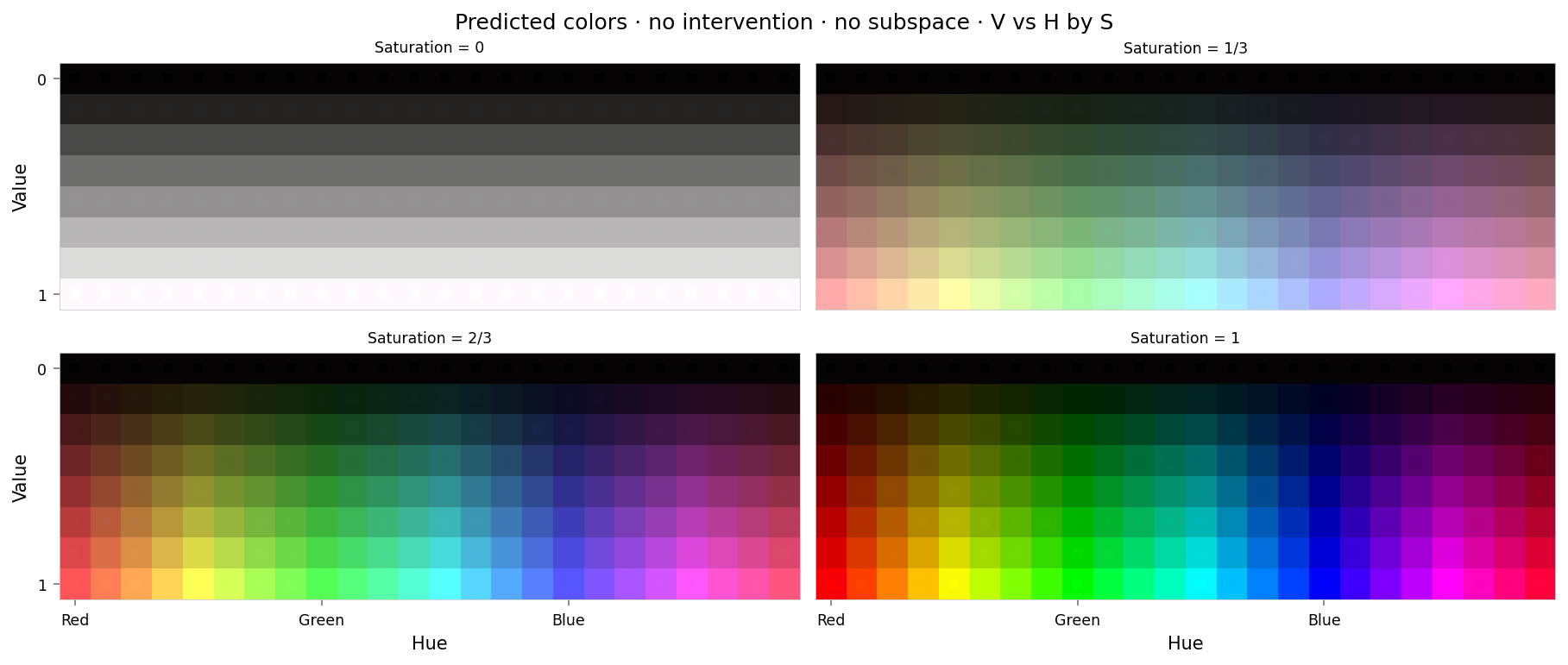
Max loss: 0.00027
Median MSE: 2.2e-05

Reconstruction loss looks about as good as last time. There's higher loss around red even without intervenion, but it's still low.

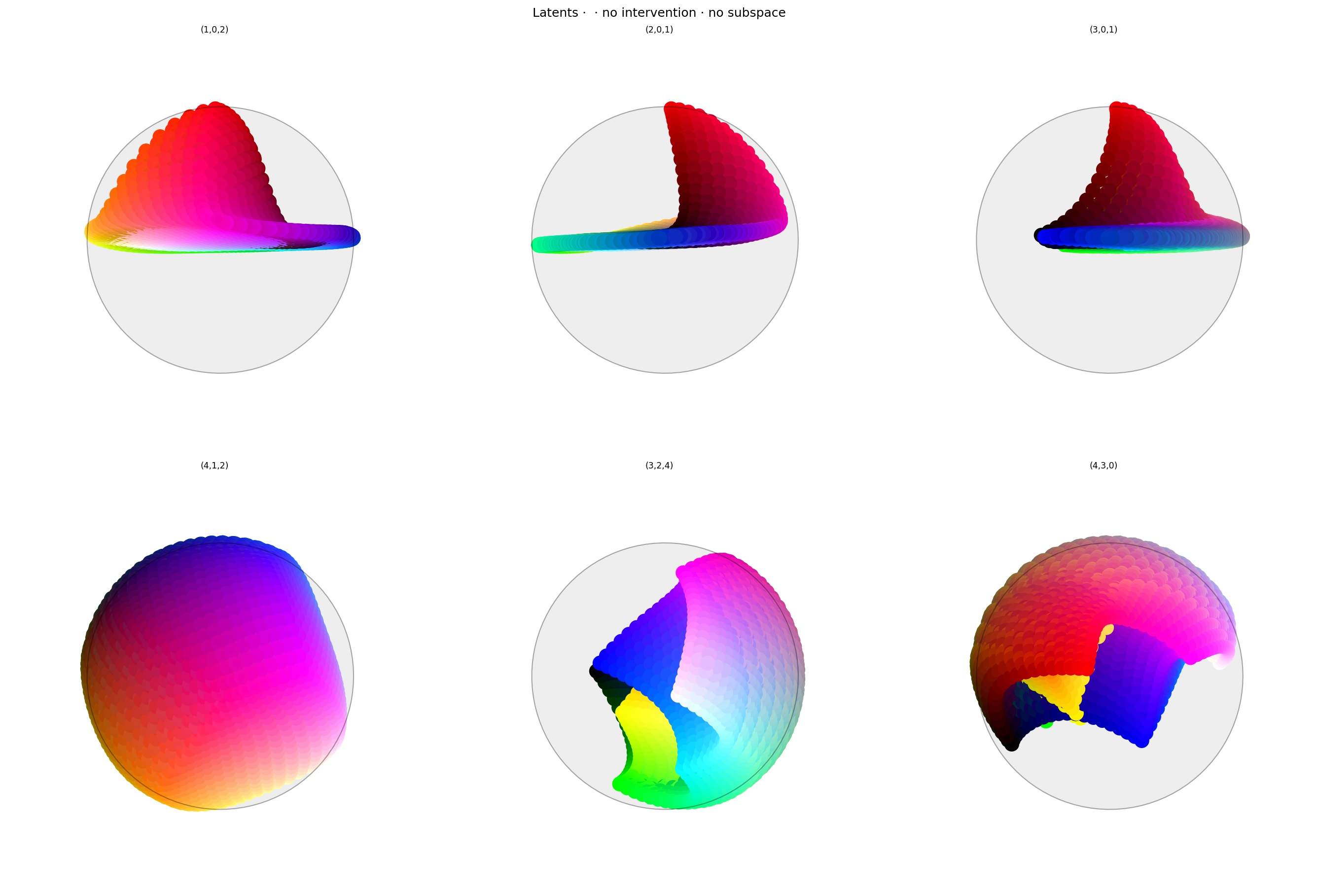
Latent space looks suprisingly good: the area opposing red is clear, and there's a pronounced collection of reds near the anchor point.

Ablation

from ex_color.surgery import ablate

ablated_model = ablate(model, 'bottleneck', [0])

from IPython.display import clear_output

tags = ['ablated', 'no intervention', 'no subspace']
hsv_out = await test(ablated_model, hsv_cube)
hd_hsv_out = await test(ablated_model, hd_hsv_cube)
rgb_out = await test(ablated_model, rgb_cube)
clear_output()

visualize_reconstructed_cube(hsv_out, tags=tags)
visualize_reconstruction_loss(hd_hsv_out, tags=tags)
visualize_latent_space(
    rgb_out,
    tags=tags,
    dims=[(1, 0, 2), (2, 0, 1), (3, 0, 1), (4, 1, 2), (3, 2, 4), (4, 3, 0)],
)

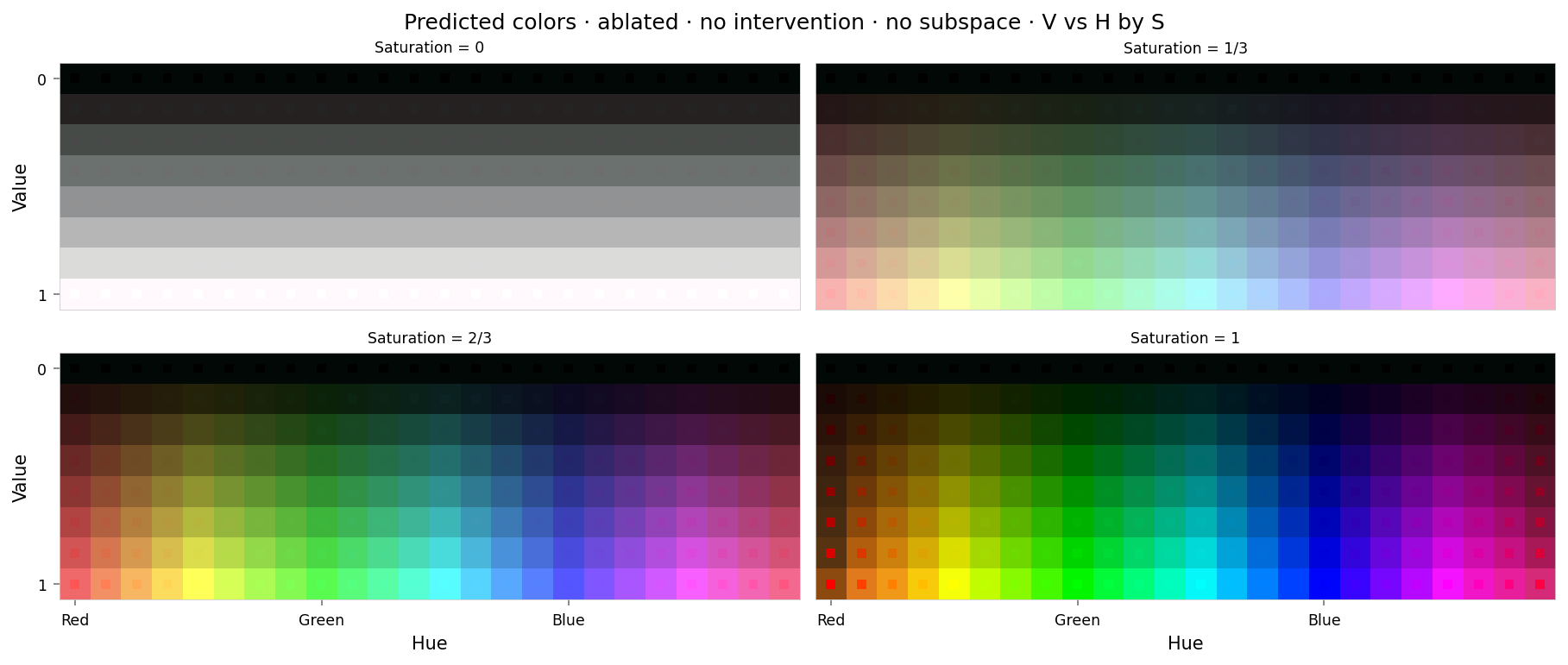
Max loss: 0.073
Median MSE: 6e-05

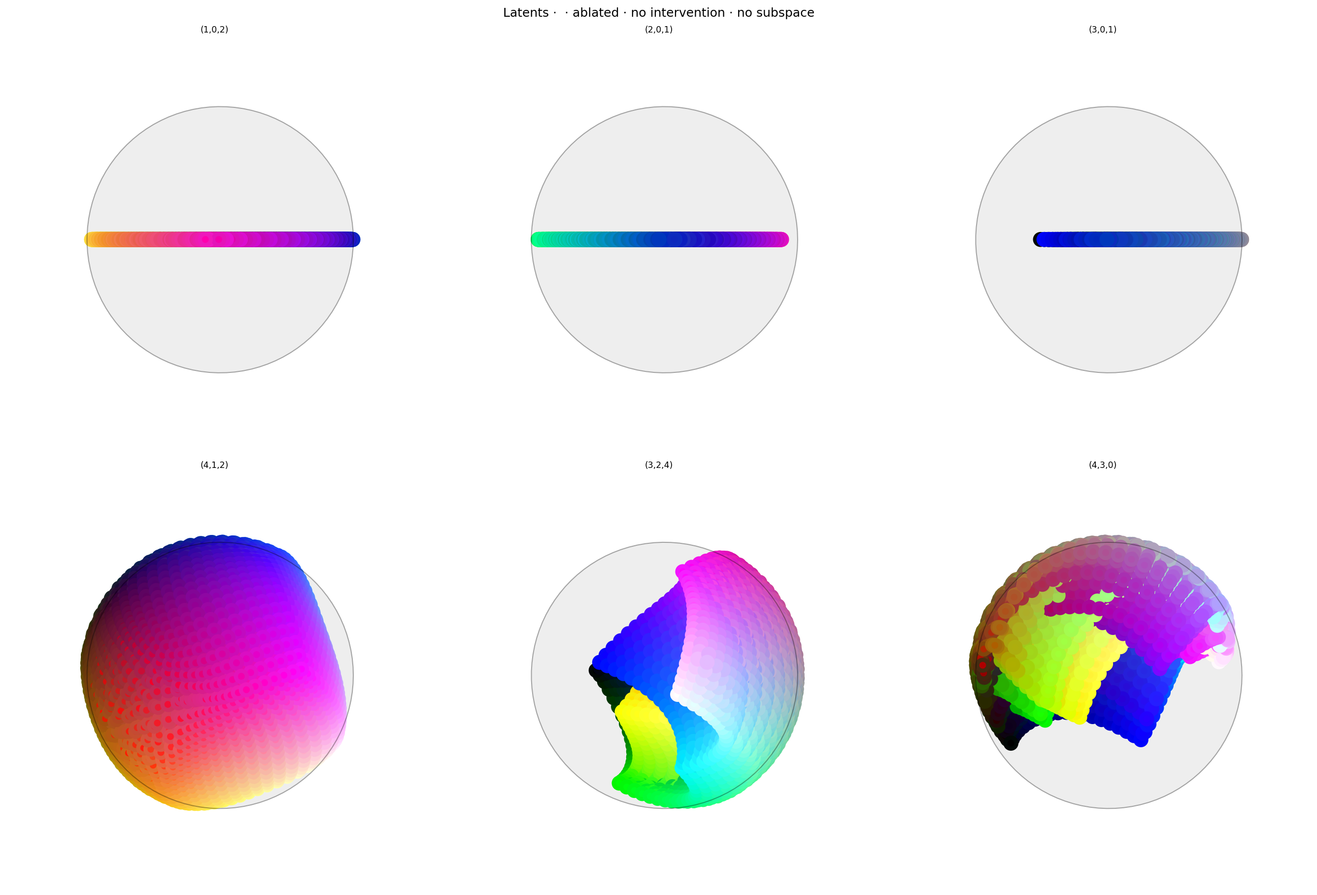
This is almost as good as last time: about 1/3 the loss for red (higher would be better), with fairly smooth falloff to the yellow and purple. There's hardly any error for other colors.

Conclusion

We can delete red without deleting cyan or other colors, even without labelling anything other than red. The error at red could be higher; perhaps that could be achieved with more hyperparameter tuning.

When we first tried this (see git history), it didn't work well: red was isolated, but the falloff toward other colors was very sharp, so there was hardly any impact on other warm colors. We fixed that by adjusting the hyperparameter schedule: instead of having Anchor and Anti-subspace in conflict the whole time, the schedule starts with a high Anti-subspace weight, and transitions to high Anchor weight around half-way through. This causes the network to section off the anchor (first) dimension at the start of training, and pulls red into that space once the manifold has already been established.