Experiment 1.8: Regularizer combinations

In Ex 1.7, we successfully imposed structure on latent space using several regularizers and weak supervision. In this experiment, we'll test what the latent space looks like with various combinations of regularizers, to see what they each contribute.

from __future__ import annotations

import logging
from utils.logging import SimpleLoggingConfig

logging_config = (
    SimpleLoggingConfig()
    .info('notebook', 'utils', 'mini', 'ex_color')
    .error('matplotlib.axes')  # Silence warnings about set_aspect
)
logging_config.apply()

# ID for tagging assets
nbid = '1.8'
# This is the logger for this notebook
log = logging.getLogger(f'notebook.{nbid}')

import modal
from mini.experiment import Experiment
from infra.requirements import freeze, project_packages

run = Experiment(f'ex-color-{nbid}')
run.image = modal.Image.debian_slim().pip_install(*freeze(all=True)).add_local_python_source(*project_packages())
run.before_each(logging_config.apply)
None

I 0.9 ut.re:   Selected 147 of 169 dependencies
I 0.9 ut.re:   Found 3 local packages: ex_color, mini, utils

Model architecture

We use the same simple 2-layer MLP autoencoder with a 4D bottleneck as in previous experiments.

import torch
import torch.nn as nn

E = 4


class ColorMLP(nn.Module):
    def __init__(self):
        super().__init__()
        # RGB input (3D) → hidden layer → bottleneck → hidden layer → RGB output
        self.encoder = nn.Sequential(
            nn.Linear(3, 16),
            nn.GELU(),
            # nn.Linear(16, 16),
            # nn.GELU(),
            nn.Linear(16, E),  # Our critical bottleneck!
        )

        self.decoder = nn.Sequential(
            nn.Linear(E, 16),
            nn.GELU(),
            # nn.Linear(16, 16),
            # nn.GELU(),
            nn.Linear(16, 3),
            nn.Sigmoid(),  # Keep RGB values in [0,1]
        )

    def forward(self, x: torch.Tensor) -> tuple[torch.Tensor, torch.Tensor]:
        # Get our bottleneck representation
        bottleneck = self.encoder(x)

        # Decode back to RGB
        output = self.decoder(bottleneck)
        return output, bottleneck

Training machinery with timeline and events

The training loop stays the same.

The train_color_model function orchestrates the training process based on a Timeline derived from the dopesheet. It handles:

• Iterating through training steps.
• Fetching the correct data loader for the current phase.
• Updating hyperparameters (like learning rate and loss weights) smoothly based on the timeline state.
• Calculating the combined loss from reconstruction and various regularizers.
• Regularizers are applied with diffent weights for each sample based on the sample labels.
• Executing the optimizer step.
• Emitting events at different points (phase start/end, pre-step, actions like 'anchor', step metrics) to trigger callbacks like plotting, recording, or updating loss terms.

from dataclasses import dataclass
from typing import Protocol, runtime_checkable
from torch import Tensor
import torch.optim as optim

from mini.temporal.timeline import TStep


@dataclass
class InferenceResult:
    outputs: Tensor
    latents: Tensor

    def detach(self):
        return InferenceResult(self.outputs.detach(), self.latents.detach())

    def clone(self):
        return InferenceResult(self.outputs.clone(), self.latents.clone())

    def cpu(self):
        return InferenceResult(self.outputs.cpu(), self.latents.cpu())


@runtime_checkable
class LossCriterion(Protocol):
    def __call__(self, data: Tensor, res: InferenceResult) -> Tensor: ...


@dataclass
class RegularizerConfig:
    """Configuration for a regularizer, including label affinities."""

    name: str
    """Matched with hyperparameter for weighting"""
    criterion: LossCriterion
    label_affinities: dict[str, float] | None
    """Maps label names to affinity strengths"""


@dataclass(eq=False, frozen=True)
class Event:
    name: str
    step: int
    model: ColorMLP
    timeline_state: TStep
    optimizer: optim.Optimizer


@dataclass(eq=False, frozen=True)
class PhaseEndEvent(Event):
    validation_data: Tensor
    inference_result: InferenceResult


@dataclass(eq=False, frozen=True)
class StepMetricsEvent(Event):
    """Event carrying metrics calculated during a training step."""

    train_batch: Tensor
    total_loss: float
    losses: dict[str, float]


class EventHandler[T](Protocol):
    def __call__(self, event: T) -> None: ...


class EventBinding[T]:
    """A class to bind events to handlers."""

    def __init__(self, event_name: str):
        self.event_name = event_name
        self.handlers: list[tuple[str, EventHandler[T]]] = []

    def add_handler(self, event_name: str, handler: EventHandler[T]) -> None:
        self.handlers.append((event_name, handler))

    def emit(self, event_name: str, event: T) -> None:
        for name, handler in self.handlers:
            if name == event_name:
                handler(event)


class EventHandlers:
    """A simple event system to allow for custom callbacks."""

    phase_start: EventBinding[Event]
    pre_step: EventBinding[Event]
    action: EventBinding[Event]
    phase_end: EventBinding[PhaseEndEvent]
    step_metrics: EventBinding[StepMetricsEvent]

    def __init__(self):
        self.phase_start = EventBinding[Event]('phase-start')
        self.pre_step = EventBinding[Event]('pre-step')
        self.action = EventBinding[Event]('action')
        self.phase_end = EventBinding[PhaseEndEvent]('phase-end')
        self.step_metrics = EventBinding[StepMetricsEvent]('step-metrics')

from functools import wraps


def periodic[T: Event](
    handler: EventHandler[T], *, interval: int, offset: int = 0, use_step: bool = True
) -> EventHandler[T]:
    """Decorator to run a handler at regular intervals."""
    i = 0

    @wraps(handler)
    def handler_wrapper(event: T):
        nonlocal i
        if use_step:
            i = event.step
        try:
            if (i + offset) % interval == 0:
                handler(event)
        finally:
            i += 1

    return handler_wrapper

Training loop

import numpy as np
import torch
from typing import Iterable, Iterator
from torch.utils.data import DataLoader
import torch.optim as optim

from mini.temporal.dopesheet import Dopesheet
from mini.temporal.timeline import Timeline


def seed_everything(seed: int):
    """Set seeds for reproducibility."""
    import random
    import numpy as np
    import torch

    random.seed(seed)
    np.random.seed(seed)
    torch.manual_seed(seed)
    if torch.cuda.is_available():
        torch.cuda.manual_seed_all(seed)
    log.debug(f'Global random seed set to {seed}')


def set_deterministic_mode(seed: int):
    """Make experiments reproducible."""
    import torch

    seed_everything(seed)
    torch.backends.cudnn.deterministic = True
    torch.backends.cudnn.benchmark = False
    log.debug('PyTorch set to deterministic mode')


def reiterate[T](it: Iterable[T]) -> Iterator[T]:
    """
    Iterates over an iterable indefinitely.

    When the iterable is exhausted, it starts over from the beginning. Unlike
    `itertools.cycle`, yielded values are not cached — so each iteration may be
    different.
    """
    while True:
        yield from it


def train_color_model(  # noqa: C901
    model: ColorMLP,
    train_loader: DataLoader,
    val_data: Tensor,
    dopesheet: Dopesheet,
    loss_criterion: LossCriterion,
    regularizers: list[RegularizerConfig],
    event_handlers: EventHandlers | None = None,
):
    if event_handlers is None:
        event_handlers = EventHandlers()

    # --- Validate inputs ---
    if 'lr' not in dopesheet.props:
        raise ValueError("Dopesheet must define the 'lr' property column.")
    # --- End Validation ---

    timeline = Timeline(dopesheet)
    optimizer = optim.Adam(model.parameters(), lr=0)
    device = next(model.parameters()).device

    train_data = iter(reiterate(train_loader))

    total_steps = len(timeline)

    for step in range(total_steps):
        # Get state *before* advancing timeline for this step's processing
        current_state = timeline.state
        current_phase_name = current_state.phase

        batch_data, batch_labels = next(train_data)
        # Should already be on device
        # batch_data = batch_data.to(device)
        # batch_labels = batch_labels.to(device)

        # --- Event Handling ---
        event_template = {
            'step': step,
            'model': model,
            'timeline_state': current_state,
            'optimizer': optimizer,
        }

        if current_state.is_phase_start:
            event = Event(name=f'phase-start:{current_phase_name}', **event_template)
            event_handlers.phase_start.emit(event.name, event)
            event_handlers.phase_start.emit('phase-start', event)

        for action in current_state.actions:
            event = Event(name=f'action:{action}', **event_template)
            event_handlers.action.emit(event.name, event)
            event_handlers.action.emit('action', event)

        event = Event(name='pre-step', **event_template)
        event_handlers.pre_step.emit('pre-step', event)

        # --- Training Step ---
        # ... (get data, update LR, zero grad, forward pass, calculate loss, backward, step) ...

        current_lr = current_state.props['lr']
        # REF_BATCH_SIZE = 32
        # lr_scale_factor = batch.shape[0] / REF_BATCH_SIZE
        # current_lr = current_lr * lr_scale_factor
        for param_group in optimizer.param_groups:
            param_group['lr'] = current_lr

        optimizer.zero_grad()

        outputs, latents = model(batch_data)
        current_results = InferenceResult(outputs, latents)

        primary_loss = loss_criterion(batch_data, current_results).mean()
        losses = {'recon': primary_loss.item()}
        total_loss = primary_loss
        zeros = torch.tensor(0.0, device=batch_data.device)

        for regularizer in regularizers:
            name = regularizer.name
            criterion = regularizer.criterion

            weight = current_state.props.get(name, 1.0)
            if weight == 0:
                continue

            if regularizer.label_affinities is not None:
                # Soft labels that indicate how much effect this regularizer has, based on its affinity with the label
                label_probs = [
                    batch_labels[k] * v
                    for k, v in regularizer.label_affinities.items()
                    if k in batch_labels  #
                ]
                if not label_probs:
                    continue

                sample_affinities = torch.stack(label_probs, dim=0).sum(dim=0)
                sample_affinities = torch.clamp(sample_affinities, 0.0, 1.0)
                if torch.allclose(sample_affinities, zeros):
                    continue
            else:
                sample_affinities = torch.ones(batch_data.shape[0], device=batch_data.device)

            per_sample_loss = criterion(batch_data, current_results)
            if len(per_sample_loss.shape) == 0:
                # If the loss is a scalar, we need to expand it to match the batch size
                per_sample_loss = per_sample_loss.expand(batch_data.shape[0])
            assert per_sample_loss.shape[0] == batch_data.shape[0], f'Loss should be per-sample OR scalar: {name}'

            # Apply sample affinities
            weighted_loss = per_sample_loss * sample_affinities

            # Apply sample importance weights
            # weighted_loss *= batch_weights

            # Calculate mean only over selected samples. If we used torch.mean, it would average over all samples, including those with 0 weight
            term_loss = weighted_loss.sum() / (sample_affinities.sum() + 1e-8)

            losses[name] = term_loss.item()
            if not torch.isfinite(term_loss):
                log.warning(f'Loss term {name} at step {step} is not finite: {term_loss}')
                continue
            total_loss += term_loss * weight

        if total_loss > 0:
            total_loss.backward()
            optimizer.step()
        # --- End Training Step ---

        # Emit step metrics event
        step_metrics_event = StepMetricsEvent(
            name='step-metrics',
            **event_template,
            train_batch=batch_data,
            total_loss=total_loss.item(),
            losses=losses,
        )
        event_handlers.step_metrics.emit('step-metrics', step_metrics_event)

        # --- Post-Step Event Handling ---
        if current_state.is_phase_end:
            # Trigger phase-end for the *current* phase
            # validation_data = batch_data
            with torch.no_grad():
                val_outputs, val_latents = model(val_data.to(device))
            event = PhaseEndEvent(
                name=f'phase-end:{current_phase_name}',
                **event_template,
                validation_data=val_data,
                inference_result=InferenceResult(val_outputs, val_latents),
            )
            event_handlers.phase_end.emit(event.name, event)
            event_handlers.phase_end.emit('phase-end', event)
        # --- End Event Handling ---

        # Advance timeline *after* processing the current step
        if step < total_steps:  # Avoid stepping past the end
            timeline.step()

    log.debug('Training finished!')

Visualization

We define an event handler that periodically draws scatter plots of the latent embeddings.

This has been refactored compared to earlier experiments: it has been split into several parts:

• evaluate_latents: The event handler (remote)
• HistoryStore: Receives latents from the event handler (local)
• history_plotter: Callback that displays the contents of the HistoryStore (local)

import typing

if typing.TYPE_CHECKING:
    from matplotlib.axes import Axes
    import numpy.typing as npt


def hide_decorations(ax: Axes, background: bool = True, ticks: bool = True, border: bool = True) -> None:
    """Remove all decorations from the axes."""
    if background:
        ax.patch.set_alpha(0)
    if ticks:
        ax.set_xticks([])
        ax.set_yticks([])
    if border:
        ax.spines['top'].set_visible(False)
        ax.spines['right'].set_visible(False)
        ax.spines['bottom'].set_visible(False)
        ax.spines['left'].set_visible(False)


def draw_latent_slice(
    ax: Axes | tuple[Axes, Axes],  # Axes for background and foreground
    latents: npt.NDArray,
    colors: npt.NDArray,
    dot_size: float = 200,
    clip_on: bool = False,
):
    """Draw a slice of the latent space."""
    from matplotlib.patches import Circle

    assert latents.ndim == 2, 'Latents should be 2D'
    assert latents.shape[1] == 2, 'Latents should have 2 dimensions'

    bg, fg = ax if isinstance(ax, tuple) else (ax, ax)
    return {
        'circ': bg.add_patch(
            Circle((0, 0), 1, facecolor='#111', edgecolor='#0000', fill=True, zorder=-1, clip_on=clip_on)
        ),
        'scatter': fg.scatter(latents[:, 0], latents[:, 1], c=colors, s=dot_size, alpha=0.7, clip_on=clip_on),
        'circ-top': fg.add_patch(Circle((0, 0), 1, edgecolor='#1118', fill=False, clip_on=clip_on)),
    }


def geometric_frame_progression(samples: int, n: int, offset: int = 10) -> npt.NDArray[np.int_]:
    """
    Generate a geometric progression of indices for sampling frames.

    Useful for creating videos of simulations in which there is more detail at the beginning.

    Args:
        samples (int): Number of samples to generate. If larger than n, it will be capped to n.
        n (int): Total number of frames to sample from.
        offset (int): Offset to apply during generation. Increase this to get more samples at the start of short sequences; larger values will result in "flatter" sequences.

    Returns:
        np.ndarray: Array of indices.
    """
    samples = min(samples, n)
    if samples <= 0:
        return np.array([], dtype=int)
    return np.unique(np.geomspace(offset, n + offset, samples, endpoint=False, dtype=int) - offset)


def bezier_frame_progression(
    samples: int,
    n: int,
    cp1: tuple[float, float],
    cp2: tuple[float, float],
    lookup_table_size: int = 200,
) -> npt.NDArray[np.int_]:
    """
    Generate a bezier curve for sampling frames.

    Args:
        samples: Number of samples to generate (inclusive upper bound).
        n: Total number of frames to sample from.
        cp1: Control point 1 (t_in, t_out), e.g. (0, 0) for a linear curve, or (0.42, 0) for a classic ease-in.
        cp2: Control point 2 (t_in, t_out), e.g. (1, 1) for a linear curve, or (0.58, 1) for a classic ease-out.
        lookup_table_size: Number of points to sample on the bezier curve. Higher values will result in smoother curves, but will take longer to compute.
    """
    from matplotlib.bezier import BezierSegment

    if samples <= 0 or n <= 0:
        return np.array([], dtype=int)
    if n == 1:
        return np.array([0], dtype=int)
    control_points = np.array([(0, 0), cp1, cp2, (1, 1)])
    bezier_curve = BezierSegment(control_points)
    t_lookup = np.linspace(0, 1, lookup_table_size)
    points_on_curve = bezier_curve(t_lookup)
    xs = points_on_curve[:, 0]
    ys = points_on_curve[:, 1]
    assert np.all(np.diff(xs) >= 0), 't is not monotonic'

    # Generate linearly spaced input times for sampling our easing function
    t_linear_input = np.linspace(0, 1, samples, endpoint=True)

    # Interpolate to get eased time:
    # For each t_linear_input (our desired "progress through animation"),
    # find the corresponding y-value on the Bézier curve (our "eased progress").
    t_eased = np.interp(t_linear_input, xs, ys)

    # Clip eased time to [0,1] in case control points caused overshoot/undershoot
    # and we want to strictly map to frame indices.
    t_eased = np.clip(t_eased, 0.0, 1.0)

    # Scale to frame indices and ensure they are unique and sorted
    frame_indices = np.round(t_eased * (n - 1)).astype(int)
    unique_indices = np.unique(frame_indices)

    return unique_indices

from typing import Callable
import matplotlib.pyplot as plt
from torch import Tensor
from IPython.display import HTML

from utils.coro import debounced
from utils.nb import save_fig


@dataclass
class LatentEvaluation:
    variant: str
    step: int
    latents: np.ndarray


def evaluate_latents(data: Tensor, variant_name: str, callback: Callable[[LatentEvaluation]]) -> EventHandler[Event]:
    # Runs remotely, in the training loop.

    def _evaluate_latents(event: Event):
        from utils.torch.training import mode

        log.debug(f'Evaluating latents at step {event.step} for variant {variant_name}')

        with torch.no_grad(), mode(event.model, 'eval'):
            _output, latents = event.model(data)

        callback(
            LatentEvaluation(
                variant=variant_name,
                step=event.step,
                latents=latents.detach().cpu().numpy(),
            )
        )

    return _evaluate_latents


class HistoryStore:
    # Exists locally
    def __init__(self):
        self.histories: dict[str, list[LatentEvaluation]] = {}
        self.observers: dict[str, list[Callable[[list[LatentEvaluation]]]]] = {}

    def __reduce__(self):
        raise RuntimeError('HistoryStore cannot be pickled - it should only exist locally')

    def add(self, latent_eval: LatentEvaluation):
        if latent_eval.variant not in self.histories:
            self.histories[latent_eval.variant] = []
        self.histories[latent_eval.variant].append(latent_eval)
        self.notify(latent_eval.variant)

    def notify(self, variant: str):
        for observer in self.observers.get(variant, []):
            observer(self.histories.get(variant, []))

    def register_observer(self, variant: str, observer: Callable[[list[LatentEvaluation]]]):
        """Register an observer for a specific variant."""
        if variant not in self.observers:
            self.observers[variant] = []
        self.observers[variant].append(observer)


@run.hither
def store_latents(store: HistoryStore):
    # Sends latents from remote to the local store.
    async def _store_latents(latent_eval: LatentEvaluation):
        store.add(latent_eval)

    return _store_latents


def safe_filename(name: str) -> str:
    """Convert a name to a safe filename by replacing non-alphanumeric characters."""
    import re

    return re.sub(r'[^a-zA-Z0-9_-]', '_', name)


def history_plotter(colors: np.ndarray, *, dim_pairs: list[tuple[int, int]], variant_name: str = ''):
    """Plot latent space"""
    from utils.nb import displayer

    # Store (phase_name, end_step, data, result) - data comes from event now
    display = displayer()
    _colors = colors.copy()

    @debounced
    def plot_history(history: list[LatentEvaluation]):
        try:
            fig = _plot_history(history, _colors, dim_pairs, variant_name)
            # display(fig)
            suffix = safe_filename(variant_name or '')
            display(
                HTML(
                    save_fig(
                        fig,
                        f'large-assets/ex-{nbid}-color-phase-history{suffix}.png',
                        alt_text='Visualizations of latent space at the end of each curriculum phase.',
                    )
                )
            )
        finally:
            plt.close()

    return plot_history


def _plot_history(
    history: list[LatentEvaluation], colors: np.ndarray, dim_pairs: list[tuple[int, int]], variant_name: str
):
    if not history:
        fig, ax = plt.subplots()
        fig.set_facecolor('#333')
        ax.set_facecolor('#222')
        ax.text(0.5, 0.5, 'Waiting...', ha='center', va='center')
        return fig

    plt.style.use('dark_background')

    # Number of dimension pairs
    num_dim_pairs = len(dim_pairs)

    # Cap the number of thumbnails to a maximum for readability
    max_thumbnails = 10
    indices = geometric_frame_progression(max_thumbnails, len(history), offset=10)
    history_to_show = [history[i] for i in indices]

    # Create figure with gridspec for flexible layout
    fig = plt.figure(figsize=(12, 5), facecolor='#333')

    # Create two separate gridspecs - one for thumbnails, one for latest state
    gs = fig.add_gridspec(3, 1, hspace=0.1, height_ratios=[0.5, 4, 1])

    # Latest state gridspec (top row) - all dimension pairs
    latest_gs = gs[1].subgridspec(2, num_dim_pairs, wspace=0, hspace=0.1, height_ratios=[0, 1])

    # Thumbnail gridspec (bottom row) - only first dimension pair
    thumbnail_gs = gs[2].subgridspec(2, max_thumbnails, wspace=0, hspace=0.1, height_ratios=[1, 0])

    # Create thumbnail axes and plot history
    for i, le in enumerate(history_to_show):
        latents, step = le.latents, le.step

        # Only plot the first dimension pair for thumbnails
        dim1, dim2 = dim_pairs[0]

        # Create title for the thumbnail as its own axes, so that it's aligned with the other titles
        axt = fig.add_subplot(thumbnail_gs[1, i])
        axt.text(
            0,
            0,
            f'{step}',
            # transform=axt.transAxes,
            horizontalalignment='center',
            verticalalignment='top',
            fontsize=7,
        )
        # Remove all decorations
        hide_decorations(axt)

        # Create thumbnail axis
        ax = fig.add_subplot(thumbnail_gs[0, i])
        ax.sharex(axt)
        draw_latent_slice(ax, latents[:, [dim1, dim2]], colors, dot_size=20)
        hide_decorations(ax)

        # Ensure square aspect ratio
        ax.set_aspect('equal')
        ax.set_adjustable('box')

    # Plot latest state
    # Get the latest data
    le = history[-1]
    latents, step = le.latents, le.step

    prev_ax = None
    for i, (dim1, dim2) in enumerate(dim_pairs):
        # Create title for the thumbnail as its own axes, so that it's aligned with the other titles
        axt = fig.add_subplot(latest_gs[0, i])
        axt.text(
            0,
            0,
            f'[{dim1}, {dim2}]',
            # transform=axt.transAxes,
            horizontalalignment='center',
            fontsize=10,
        )
        hide_decorations(axt)

        # Plot
        ax = fig.add_subplot(latest_gs[1, i])
        ax.sharex(axt)
        if prev_ax is not None:
            ax.sharey(prev_ax)
        prev_ax = ax
        draw_latent_slice(ax, latents[:, [dim1, dim2]], colors)
        hide_decorations(ax)

        # Ensure square aspect ratio
        ax.set_aspect('equal')
        ax.set_adjustable('box')

    # Add overall title
    fig.suptitle(f'Latent space — step {step}', fontsize=12, color='white')

    # Subtitle
    ax = fig.add_subplot(gs[0])
    ax.text(
        0.5,
        1,
        f'{variant_name}',
        horizontalalignment='center',
        verticalalignment='top',
        fontsize='small',
        color='white',
    )
    hide_decorations(ax)

    # Use subplots_adjust instead of tight_layout to avoid warnings
    fig.subplots_adjust(top=0.9, bottom=0.1, left=0.1, right=0.95)

    return fig

Hyperparameter dopesheet

As in previous experiments, we'll define a dopesheet (timeline) to allow hyperparameters to vary over time. Not all of the hyperparameters will be used for each run: it depends on which regularizers are in use.

import re

from IPython.display import display, HTML
from matplotlib.figure import Figure

from mini.temporal.vis import plot_timeline, realize_timeline, ParamGroup
from mini.temporal.dopesheet import Dopesheet
from mini.temporal.timeline import Timeline
from utils.nb import save_fig


line_styles = [
    (re.compile(r'^data-'), {'linewidth': 5, 'zorder': -1, 'alpha': 0.5}),
    # (re.compile(r'-(anchor|norm)$'), {'linewidth': 2, 'linestyle': (0, (8, 1, 1, 1))}),
]


def load_dopesheet():
    return Dopesheet.from_csv(f'ex-{nbid}-dopesheet.csv')


def plot_dopesheet(dopesheet: Dopesheet):
    # display(Markdown(f"""## Parameter schedule ({variant})\n{dopesheet.to_markdown()}"""))

    timeline = Timeline(dopesheet)
    history_df = realize_timeline(timeline)
    keyframes_df = dopesheet.as_df()

    groups = (
        ParamGroup(
            name='',
            params=[p for p in dopesheet.props if p not in {'lr'}],
            height_ratio=2,
        ),
        ParamGroup(
            name='',
            params=[p for p in dopesheet.props if p in {'lr'}],
            height_ratio=1,
        ),
    )
    fig, ax = plot_timeline(history_df, keyframes_df, groups, line_styles=line_styles)
    # Add assertion to satisfy type checker
    assert isinstance(fig, Figure), 'plot_timeline should return a Figure'
    display(
        HTML(
            save_fig(
                fig,
                f'large-assets/ex-{nbid}-color-timeline.png',
                alt_text='Line chart showing the hyperparameter schedule over time.',
            )
        )
    )


dopesheet = load_dopesheet()

Loss functions and regularizers

As in earlier experiments, we use mean squared error for the main reconstruction loss (loss-recon), and regularizers that encourage embeddings of unit length, and for primary colors to be on the plane of the first two dimensions. Regularizers can have different strengths depending on which sample they're evaluating. See Labelling and Train below.

from torch import linalg as LA

from ex_color.data.color_cube import ColorCube
from ex_color.data.cyclic import arange_cyclic


def objective(fn):
    """Adapt loss function to look like a regularizer"""

    def wrapper(data: Tensor, res: InferenceResult) -> Tensor:
        loss = fn(data, res.outputs)
        # Reduce element-wise loss to per-sample loss by averaging over feature dimensions
        if loss.ndim > 1:
            # Calculate mean over all dimensions except the first (batch) dimension
            reduce_dims = tuple(range(1, loss.ndim))
            loss = torch.mean(loss, dim=reduce_dims)
        return loss

    return wrapper


def unitarity(data: Tensor, res: InferenceResult) -> Tensor:
    """Regularize latents to have unit norm (vectors of length 1)"""
    norms = LA.vector_norm(res.latents, dim=-1)
    # Return per-sample loss, shape [B]
    return (norms - 1.0) ** 2


def planarity(data: Tensor, res: InferenceResult) -> Tensor:
    """Regularize latents to be planar in the first two channels (so zero in other channels)"""
    if res.latents.shape[1] <= 2:
        # No dimensions beyond the first two, return zero loss per sample
        return torch.zeros(res.latents.shape[0], device=res.latents.device)
    # Sum squares across the extra dimensions for each sample, shape [B]
    return torch.sum(res.latents[:, 2:] ** 2, dim=-1)

Pin (anchor)

This regularizer causes certain samples to be attracted to a certain anchor point.

class Pin(LossCriterion):
    def __init__(self, anchor_point: Tensor):
        self.anchor_point = anchor_point

    def __call__(self, data: Tensor, res: InferenceResult) -> Tensor:
        """
        Regularize latents to be close to the anchor point.

        Returns:
            loss: Per-sample loss, shape [B].
        """
        # Calculate squared distances to the anchor
        anchor_point = self.anchor_point.to(res.latents.device)
        sq_dists = torch.sum((res.latents - anchor_point) ** 2, dim=-1)  # [B]
        return sq_dists

Separate

The unitarity term encourages embeddings to have unit length, but by default, that causes them to bunch up on one side of the hypersphere. To counter that, Separate adds a repulsive force along the surface of the hypersphere.

from types import EllipsisType


class Separate(LossCriterion):
    """Regularize latents to be rotationally separated from each other."""

    def __init__(self, channels: tuple[int, ...] | EllipsisType = ..., power: float = 1.0, shift: bool = True):
        self.channels = channels
        self.power = power
        self.shift = shift

    def __call__(self, data: Tensor, res: InferenceResult) -> Tensor:
        embeddings = res.latents[:, self.channels]  # [B, C]

        # Normalize to unit hypersphere, so it's only the angular distance that matters
        embeddings = embeddings / (torch.norm(embeddings, dim=-1, keepdim=True) + 1e-8)

        # Find the angular distance as cosine similarity
        cos_sim = torch.matmul(embeddings, embeddings.T)  # [B, B]

        # Nullify self-repulsion.
        # We can't use torch.eye, because some points in the batch may be duplicates due to the use of random sampling with replacement.
        cos_sim[torch.isclose(cos_sim, torch.ones_like(cos_sim))] = 0.0
        if self.shift:
            # Shift the cosine similarity to be in the range [0, 1]
            cos_sim = (cos_sim + 1.0) / 2.0

        # Sum over all other points
        return torch.sum(cos_sim**self.power, dim=-1)  # [B]

Data loading, sampling, and event handling

Here we set up:

• Datasets: Define the datasets used (primary/secondary colors, full color grid).
• Sampler: Use DynamicWeightedRandomBatchSampler for the full dataset. Its weights are updated by the update_sampler_weights callback, which responds to the data-fraction parameter from the dopesheet. This smoothly shifts the sampling focus from highly vibrant colors early on to the full range of colors later.
• Recorders: ModelRecorder and MetricsRecorder are event handlers that save the model state and loss values at each step.
• Event bindings: Connect event handlers to specific events (e.g., plotter to phase-end, reg_anchor.on_anchor to action:anchor, recorders to pre-step and step-metrics).
• Training execution: Finally, call train_color_model with the model, datasets, dopesheet, loss criteria, and configured event handlers.

Recorders

import numpy as np
import torch.nn as nn


class ModelRecorder(EventHandler):
    """Event handler to record model parameters."""

    history: list[tuple[int, dict[str, Tensor]]]
    """A list of tuples (step, state_dict) where state_dict is a copy of the model's state dict."""

    def __init__(self):
        self.history = []

    def __call__(self, event: Event):
        # Get a *copy* of the state dict and move it to the CPU
        # so we don't hold onto GPU memory or track gradients unnecessarily.
        model_state = {k: v.cpu().clone() for k, v in event.model.state_dict().items()}
        self.history.append((event.step, model_state))
        log.debug(f'Recorded model state at step {event.step}')


class BatchRecorder(EventHandler):
    """Event handler to record the exact batches used at each step."""

    history: list[tuple[int, Tensor]]
    """A list of tuples (step, train_batch)."""

    def __init__(self):
        self.history = []

    def __call__(self, event: StepMetricsEvent):
        if not isinstance(event, StepMetricsEvent):
            log.warning(f'BatchRecorder received unexpected event type: {type(event)}')
            return
        self.history.append((event.step, event.train_batch.cpu().clone()))
        log.debug(f'Recorded batch at step {event.step}')


class MetricsRecorder(EventHandler):
    """Event handler to record training metrics."""

    history: list[tuple[int, float, dict[str, float]]]
    """A list of tuples (step, total_loss, losses_dict)."""

    def __init__(self):
        self.history = []

    def __call__(self, event: StepMetricsEvent):
        if not isinstance(event, StepMetricsEvent):
            log.warning(f'MetricsRecorder received unexpected event type: {type(event)}')
            return

        self.history.append((event.step, event.total_loss, event.losses.copy()))
        log.debug(f'Recorded metrics at step {event.step}: loss={event.total_loss:.4f}')

Labelling

Labelling remains the same.

The training dataset has a fixed and somewhat small size. We want to simulate noisy labels — e.g. RGB 1,0,0 should not always be labelled "red", and colors close to red should also sometimes attract that label.

Here we define a collation function for use with DataLoader. It takes a batch and produces labels for the samples on the fly, which means the model may see identical samples with different labels during training.

Labels are assigned based on proximity to certain colors. The raw distance is not used; instead it is raised to a power to sharpen the association, and weaken the label for colors that are futher away. Initially the labels are smooth $(0..1)$. They are then converted to binary $\lbrace 0,1 \rbrace$ by comparison to random numbers.

The label "red" (i.e. proximity to pure red) is calculated as:

$$\text{red} = \left(r - \frac{rg}{2} - \frac{rb}{2}\right) ^{10}$$

While "vibrant" (proximity to any pure hue) is:

$$\text{vibrant} = \left(s \times v\right)^{100}$$

Where $r$, $g$, and $b$ are the red, green, and blue channels, and $s$ and $v$ are the saturation and value — all of which are real numbers between 0 and 1.

import torch
from torch.utils.data import DataLoader, TensorDataset, WeightedRandomSampler
from torch.utils.data.dataloader import default_collate


def generate_color_labels(data: Tensor, vibrancies: Tensor) -> dict[str, Tensor]:
    """
    Generate label probabilities based on RGB values.

    Args:
        data: Batch of RGB values [B, 3]

    Returns:
        Dictionary mapping label names to probabilities str -> [B]
    """
    labels: dict[str, Tensor] = {}

    # Labels are assigned based on proximity to certain colors.
    # Distance is raised to a power to sharpen the association (i.e. weaken the label for colors that are futher away).

    # Proximity to primary colors
    r, g, b = data[:, 0], data[:, 1], data[:, 2]
    labels['red'] = (r * (1 - g / 2 - b / 2)) ** 10
    # labels['green'] = g * (1 - r / 2 - b / 2)
    # labels['blue'] = b * (1 - r / 2 - g / 2)

    # Proximity to any fully-saturated, fully-bright color
    labels['vibrant'] = vibrancies**100

    return labels


def collate_with_generated_labels(
    batch,
    *,
    soft: bool = True,
    scale: dict[str, float] | None = None,
) -> tuple[Tensor, dict[str, Tensor]]:
    """
    Custom collate function that generates labels for the samples.

    Args:
        batch: A list of ((data_tensor,), index_tensor) tuples from TensorDataset.
               Note: TensorDataset wraps single tensors in a tuple.
        soft: If True, return soft labels (0..1). Otherwise, return hard labels (0 or 1).
        scale: Linear scaling factors for the labels (applied before discretizing).

    Returns:
        A tuple: (collated_data_tensor, collated_labels_tensor)
    """
    # Separate data and indices
    # TensorDataset yields tuples like ((data_point_tensor,), index_scalar_tensor)
    data_tuple_list = [item[0] for item in batch]  # List of (data_tensor,) tuples
    vibrancies = [item[1] for item in batch]

    # Collate the data points using the default collate function
    # default_collate handles the list of (data_tensor,) tuples correctly
    collated_data = default_collate(data_tuple_list)
    vibrancies = default_collate(vibrancies)
    label_probs = generate_color_labels(collated_data, vibrancies)
    for k, v in (scale or {}).items():
        label_probs[k] = label_probs[k] * v

    if soft:
        # Return the probabilities directly
        return collated_data, label_probs
    else:
        # Sample labels stochastically
        labels = {k: discretize(v) for k, v in label_probs.items()}
        return collated_data, labels


def discretize(probs: Tensor) -> Tensor:
    """
    Discretize probabilities into binary labels.

    Args:
        probs: Tensor of probabilities [B]

    Returns:
        Tensor of binary labels [B]
    """
    # Sample from a uniform distribution
    rand = torch.rand_like(probs)
    return (rand < probs).float()  # Convert to float for compatibility with loss functions

Datasets

Like Ex 1.7, we'll train on the HSV cube (with RGB values) and validate with the RGB cube. We train on the whole HSV cube right from the start, with a sampling bias to prevent too much importance being given to dark and desaturated colors (which are over-represented in the training data).

from functools import partial
from ex_color.data.cube_sampler import vibrancy


def prep_data():
    hsv_cube = ColorCube.from_hsv(
        h=arange_cyclic(step_size=10 / 360),
        s=np.linspace(0, 1, 10),
        v=np.linspace(0, 1, 10),
    )
    hsv_tensor = torch.tensor(hsv_cube.rgb_grid.reshape(-1, 3), dtype=torch.float32)
    vibrancy_tensor = torch.tensor(vibrancy(hsv_cube).flatten(), dtype=torch.float32)
    hsv_dataset = TensorDataset(hsv_tensor, vibrancy_tensor)

    labeller = partial(
        collate_with_generated_labels,
        soft=False,  # Use binary labels (stochastic) to simulate the labelling of internet text
        scale={'red': 0.5, 'vibrant': 0.5},
    )
    # Desaturated and dark colors are over-represented in the cube, so we use a weighted sampler to balance them out
    hsv_loader = DataLoader(
        hsv_dataset,
        batch_size=64,
        sampler=WeightedRandomSampler(
            weights=hsv_cube.bias.flatten().tolist(),
            num_samples=len(hsv_dataset),
            replacement=True,
        ),
        collate_fn=labeller,
    )

    rgb_cube = ColorCube.from_rgb(
        r=np.linspace(0, 1, 8),
        g=np.linspace(0, 1, 8),
        b=np.linspace(0, 1, 8),
    )
    rgb_tensor = torch.tensor(rgb_cube.rgb_grid.reshape(-1, 3), dtype=torch.float32)
    return hsv_loader, rgb_tensor

Train

Regularizer configuration

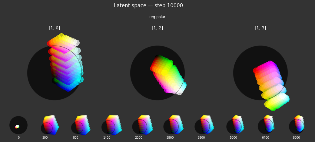
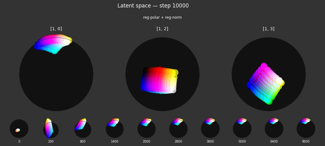
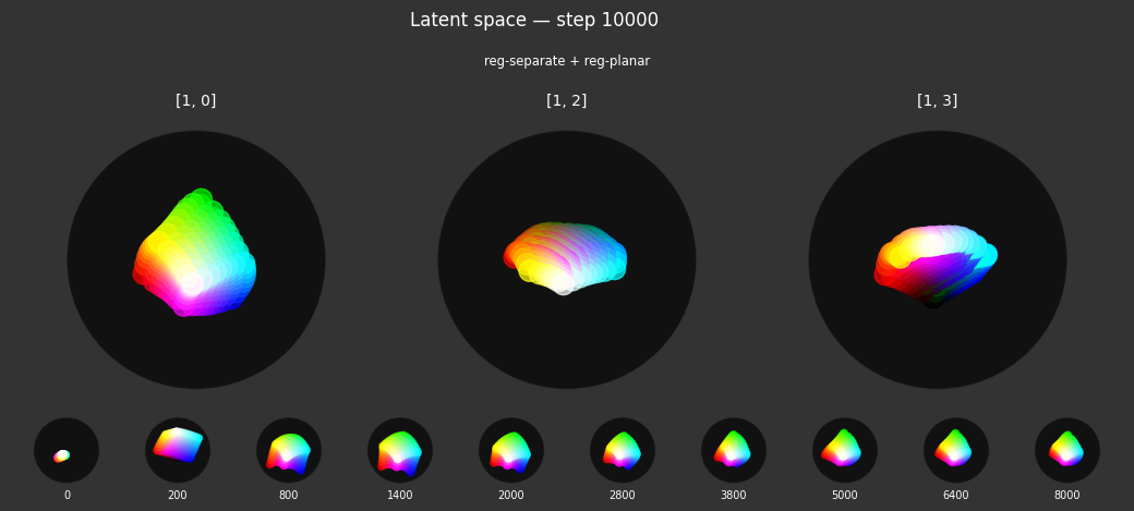
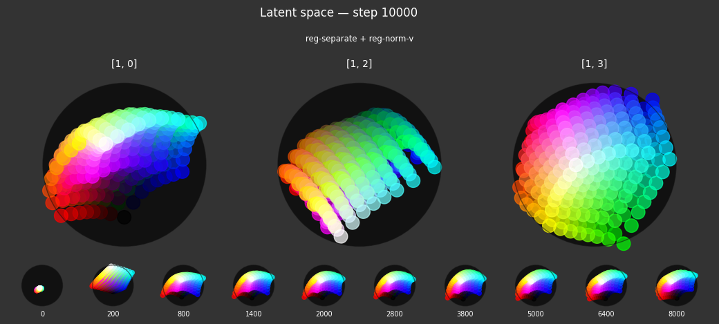
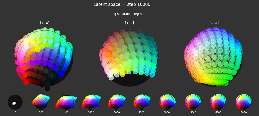
The training process can use several regularizers, each designed to impose specific structural properties on the latent space. In this experiment, we will test various combinations of these regularizers to understand their individual and combined effects.

These are the available regularizers:

• reg-polar: Concept anchor for the color red.

  • Criterion: Pin to the latent coordinate (1, 0, 0, 0). This encourages specific embeddings to move towards this "polar" anchor point.
  • Label affinity: {'red': 1.0}. This regularizer is fully active (strength 1.0) for samples that are labeled as 'red'. Its goal is to anchor the concept of "red" to a specific location in the latent space.

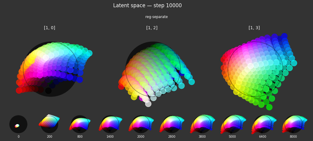
• reg-separate: Encourages the full space to be used.

  • Criterion: Separate (with power=10.0, shift=False). This term encourages all embeddings in a batch to be rotationally distinct from each other. It calculates the cosine similarity between embeddings and applies a repulsive force, powered up to make the effect greater for pairs of points that are very close. The shift=False means it uses the raw cosine similarity (ranging from -1 to 1).
  • Label affinity: None. This regularizer applies equally to all samples in the batch, irrespective of their labels, aiming for a general separation of all learned representations.

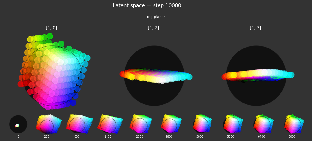
• reg-planar: Defines a "hue" plane, onto which the color wheel should emerge.

  • Criterion: planarity. This penalizes embeddings for having non-zero values in latent dimensions beyond the first two (i.e., dimensions 2 and 3, given a 4D latent space). It encourages these embeddings to lie on the plane defined by the first two latent dimensions.
  • Label affinity: {'vibrant': 1.0}. This regularizer is fully active for samples labeled as 'vibrant'. The idea is to map vibrant, pure hues primarily onto a 2D manifold within the latent space, potentially representing a color wheel.

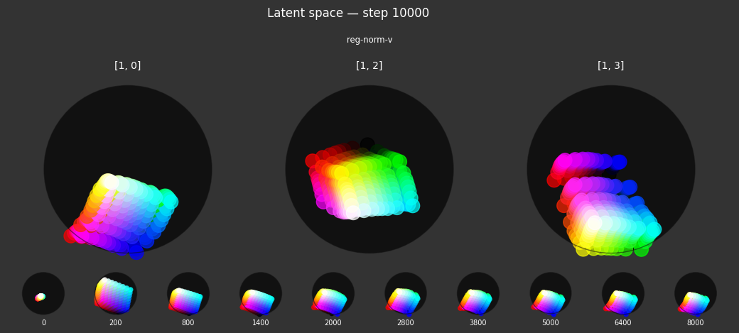
• reg-norm-v: Encourages a circular color wheel, rather than hexagonal.

  • Criterion: unitarity. This encourages the latent embeddings to have a norm (length) of 1, pushing them towards the surface of a hypersphere.
  • Label affinity: {'vibrant': 1.0}. This normalization is specifically applied with full strength to samples labeled as 'vibrant'. This works in conjunction with reg-planar to organize vibrant colors on a 2D spherical surface.

• reg-norm: Encourages embeddings to lie on the surface of a hypersphere, so they can be compared with cosine distance alone.

  • Criterion: unitarity. This also encourages latent embeddings to have a unit norm.
  • Label affinity: None. This regularizer applies the unit norm constraint to all samples in the batch, regardless of their labels. This ensures that even non-vibrant colors are normalized, contributing to a more uniform distribution of embeddings on the hypersphere.

ALL_REGULARIZERS = [
    RegularizerConfig(
        name='reg-polar',
        criterion=Pin(torch.tensor([1, 0, 0, 0], dtype=torch.float32)),
        label_affinities={'red': 1.0},
    ),
    RegularizerConfig(
        name='reg-separate',
        criterion=Separate(power=10.0, shift=False),
        label_affinities=None,
    ),
    RegularizerConfig(
        name='reg-planar',
        criterion=planarity,
        label_affinities={'vibrant': 1.0},
    ),
    RegularizerConfig(
        name='reg-norm-v',
        criterion=unitarity,
        label_affinities={'vibrant': 1.0},
    ),
    RegularizerConfig(
        name='reg-norm',
        criterion=unitarity,
        label_affinities=None,
    ),
]


@run.thither(max_containers=16)
async def train(
    dopesheet: Dopesheet,
    regularizers: list[RegularizerConfig],
    variant_name: str,
    store_latents: Callable[[LatentEvaluation], None],
):
    """Train the model with the given dopesheet and variant."""
    log.info(f'Training with: {[r.name for r in regularizers]}')
    # recorder = ModelRecorder()
    metrics_recorder = MetricsRecorder()
    # batch_recorder = BatchRecorder()

    seed = 0
    set_deterministic_mode(seed)

    hsv_loader, rgb_tensor = prep_data()
    model = ColorMLP()
    total_params = sum(p.numel() for p in model.parameters() if p.requires_grad)
    log.debug(f'Model initialized with {total_params:,} trainable parameters.')

    event_handlers = EventHandlers()
    # event_handlers.pre_step.add_handler('pre-step', recorder)
    event_handlers.step_metrics.add_handler('step-metrics', metrics_recorder)
    # event_handlers.step_metrics.add_handler('step-metrics', batch_recorder)

    # plotter = PhasePlotter(rgb_tensor, dim_pairs=[(1, 0), (1, 2), (1, 3)], variant_name=variant_name)
    event_handlers.pre_step.add_handler(
        'pre-step',
        periodic(
            evaluate_latents(rgb_tensor, variant_name, store_latents),
            interval=200,
        ),
    )

    train_color_model(
        model,
        hsv_loader,
        rgb_tensor,
        dopesheet,
        # loss_criterion=objective(nn.MSELoss(reduction='none')),  # No reduction; allows per-sample loss weights
        loss_criterion=objective(nn.MSELoss()),
        regularizers=regularizers,
        event_handlers=event_handlers,
    )

    return metrics_recorder

import itertools
from asyncio import Task, TaskGroup

all_regs = ALL_REGULARIZERS
all_combinations = list(itertools.chain(*(itertools.combinations(all_regs, i) for i in range(1, len(all_regs) + 1))))

combinations = all_combinations[:]  # For testing, select a subset
log.info(f'Running {len(combinations):d}/{len(all_combinations):d} combinations of {len(all_regs)} regularizers.')

_, rgb_tensor = prep_data()
colors = rgb_tensor.cpu().numpy()
history_store = HistoryStore()

tasks: dict[str, Task[MetricsRecorder]] = {}
async with run(shutdown_timeout=300), store_latents(history_store) as _store_latents, TaskGroup() as tg:
    for combo in combinations:
        dopesheet = load_dopesheet()
        combo_list = list(combo)
        combo_name = ' + '.join(r.name for r in combo_list)
        plotter = history_plotter(colors=colors, dim_pairs=[(1, 0), (1, 2), (1, 3)], variant_name=combo_name)
        history_store.register_observer(variant=combo_name, observer=plotter)
        task = tg.create_task(train(dopesheet, combo_list, variant_name=combo_name, store_latents=_store_latents))
        tasks[combo_name] = task

results: dict[str, MetricsRecorder] = {k: t.result() for k, t in tasks.items()}

# metrics = results[list(results.keys())[-1]]

I 5.8 no.1.8:  Running 31/31 combinations of 5 regularizers.
I 0.1 no.1.8:  Training with: ['reg-polar']
I 0.1 no.1.8:  Training with: ['reg-separate']
I 0.0 no.1.8:  Training with: ['reg-planar']
I 0.0 no.1.8:  Training with: ['reg-norm-v']
I 0.0 no.1.8:  Training with: ['reg-norm']
I 0.0 no.1.8:  Training with: ['reg-polar', 'reg-separate']
I 0.0 no.1.8:  Training with: ['reg-polar', 'reg-planar']
I 0.0 no.1.8:  Training with: ['reg-polar', 'reg-norm-v']

I 24.0 no.1.8: Training with: ['reg-polar', 'reg-norm']
I 24.4 no.1.8: Training with: ['reg-separate', 'reg-planar']
I 25.0 no.1.8: Training with: ['reg-separate', 'reg-norm-v']
I 29.8 no.1.8: Training with: ['reg-separate', 'reg-norm']

I 37.8 no.1.8: Training with: ['reg-planar', 'reg-norm-v']

I 43.5 no.1.8: Training with: ['reg-planar', 'reg-norm']
I 44.8 no.1.8: Training with: ['reg-norm-v', 'reg-norm']
I 45.7 no.1.8: Training with: ['reg-polar', 'reg-separate', 'reg-planar']
I 51.3 no.1.8: Training with: ['reg-polar', 'reg-separate', 'reg-norm-v']
I 51.0 no.1.8: Training with: ['reg-polar', 'reg-separate', 'reg-norm']

I 59.6 no.1.8: Training with: ['reg-polar', 'reg-planar', 'reg-norm-v']
I 70.4 no.1.8: Training with: ['reg-polar', 'reg-planar', 'reg-norm']

I 71.4 no.1.8: Training with: ['reg-polar', 'reg-norm-v', 'reg-norm']
I 72.7 no.1.8: Training with: ['reg-separate', 'reg-planar', 'reg-norm-v']
I 75.6 no.1.8: Training with: ['reg-separate', 'reg-planar', 'reg-norm']
I 78.0 no.1.8: Training with: ['reg-separate', 'reg-norm-v', 'reg-norm']
I 78.8 no.1.8: Training with: ['reg-planar', 'reg-norm-v', 'reg-norm']

I 80.8 no.1.8: Training with: ['reg-polar', 'reg-separate', 'reg-planar', 'reg-norm-v']
I 95.2 no.1.8: Training with: ['reg-polar', 'reg-separate', 'reg-planar', 'reg-norm']

I 104.0 no.1.8:Training with: ['reg-polar', 'reg-separate', 'reg-norm-v', 'reg-norm']

I 106.1 no.1.8:Training with: ['reg-polar', 'reg-planar', 'reg-norm-v', 'reg-norm']
I 106.3 no.1.8:Training with: ['reg-separate', 'reg-planar', 'reg-norm-v', 'reg-norm']
I 114.4 no.1.8:Training with: ['reg-polar', 'reg-separate', 'reg-planar', 'reg-norm-v', 'reg-norm']

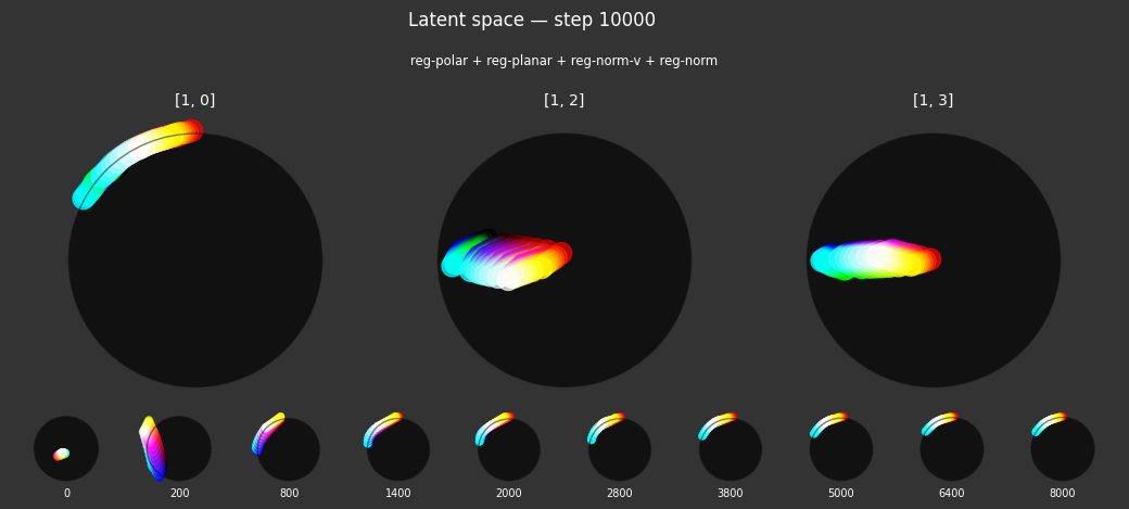
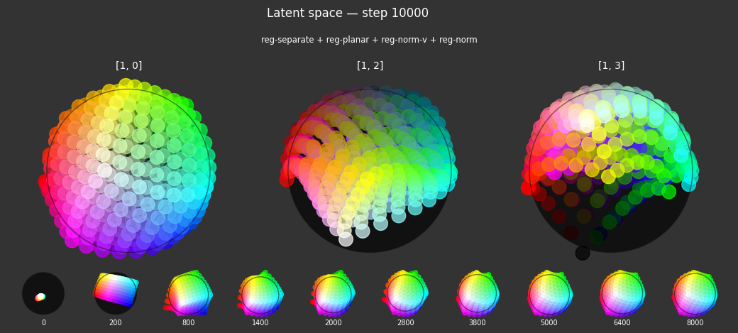
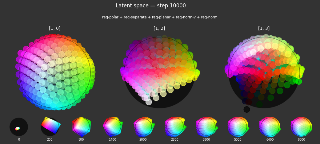
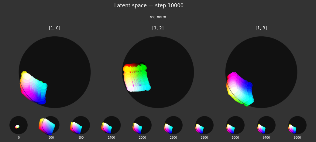
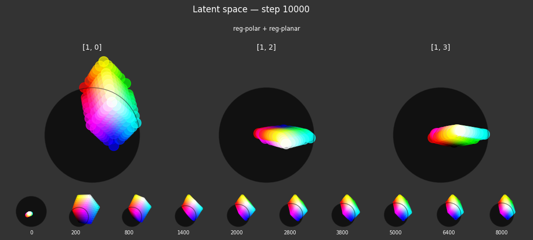
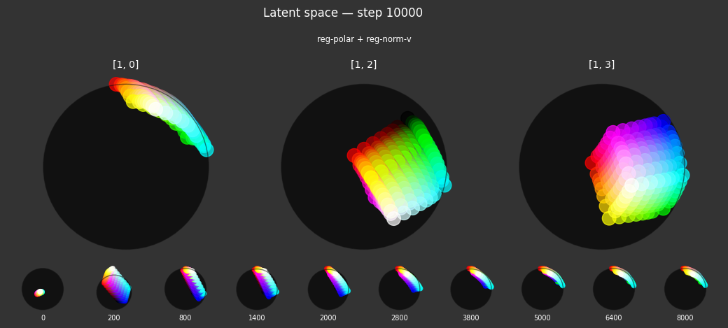
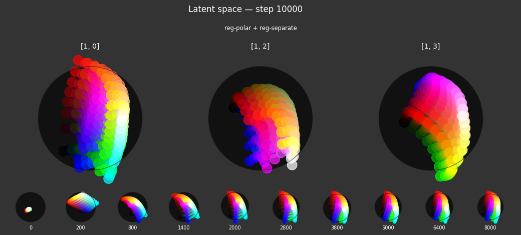
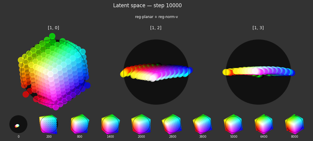
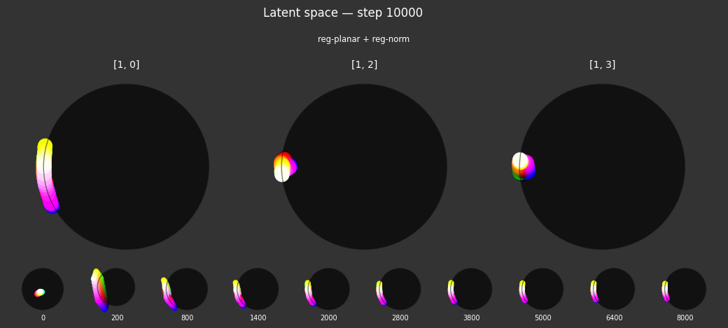
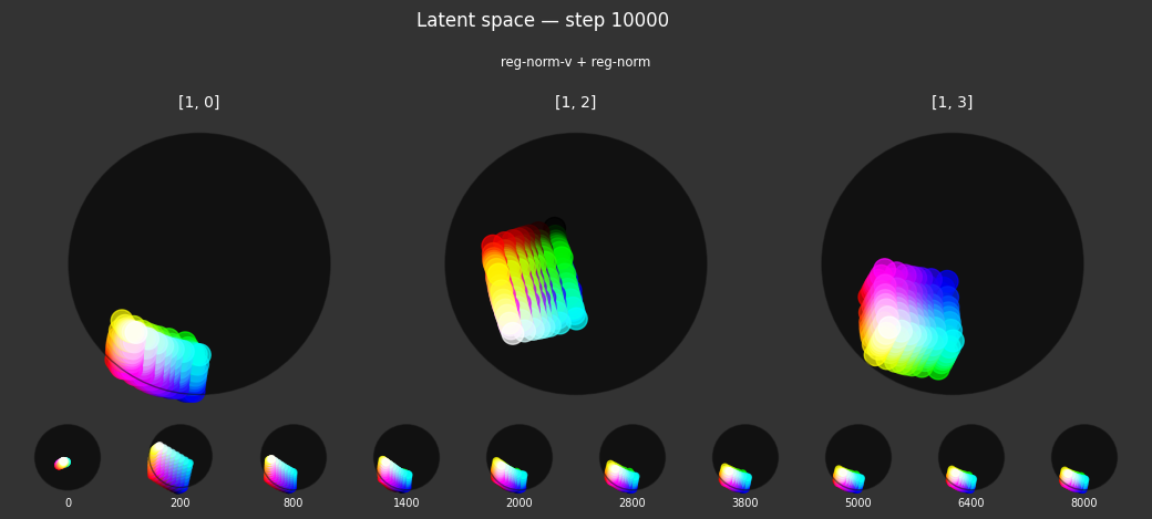
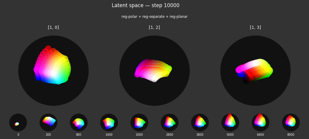
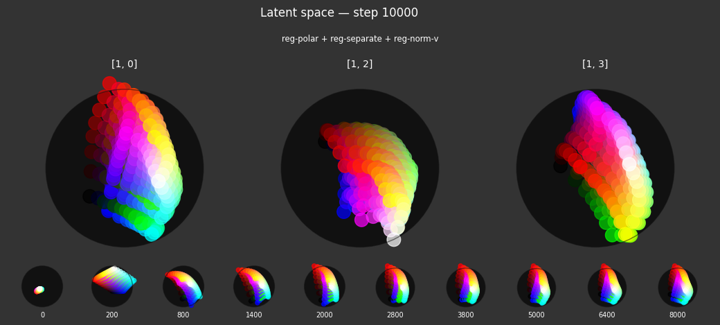
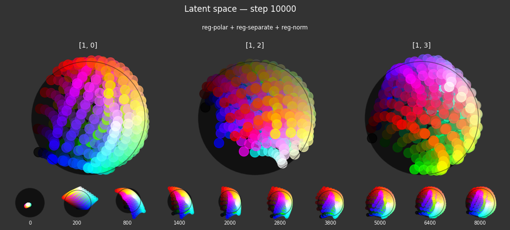
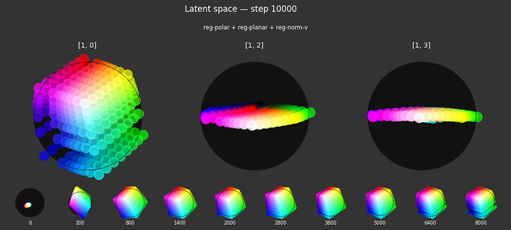
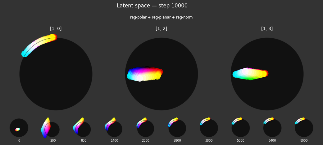
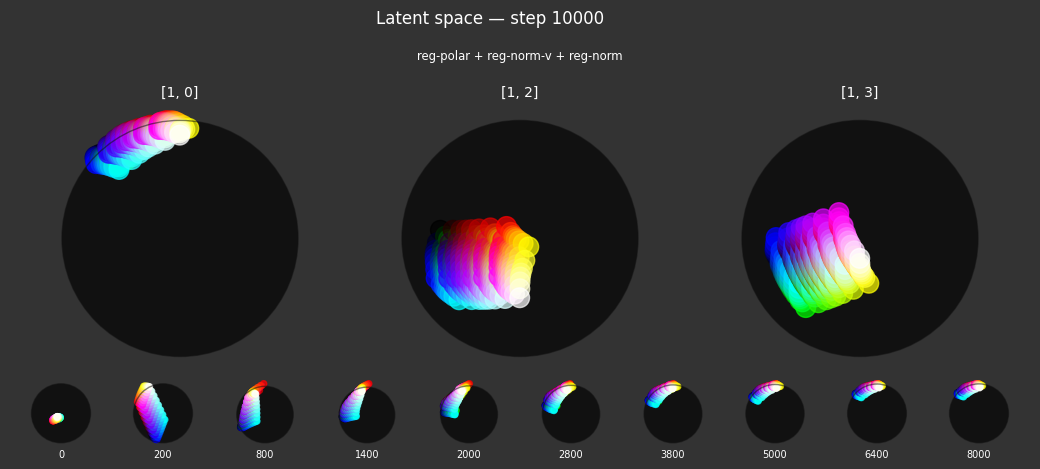
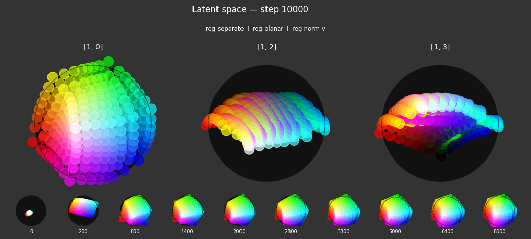
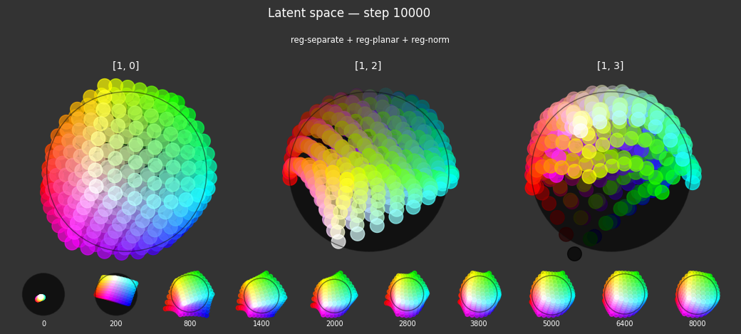
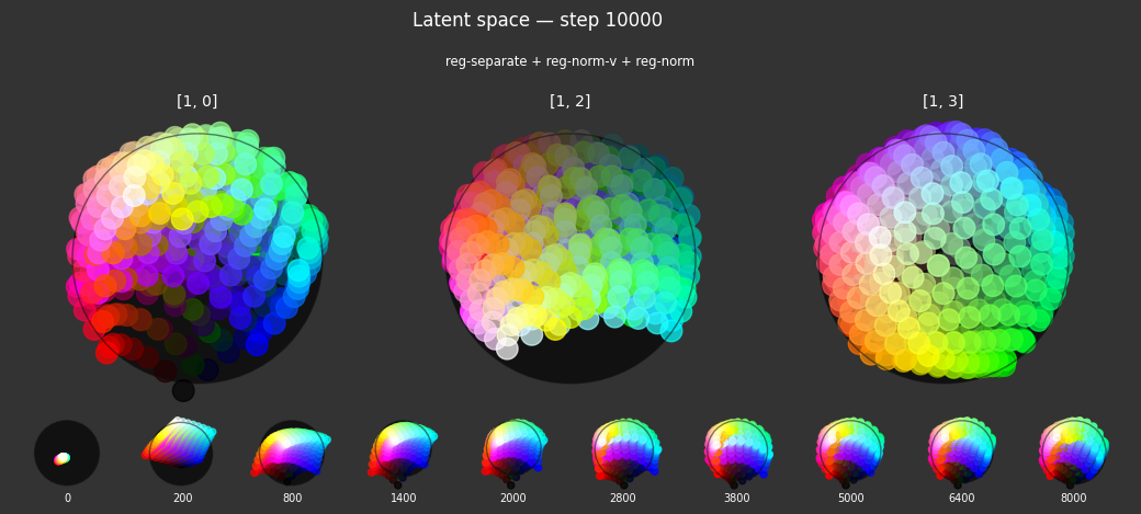
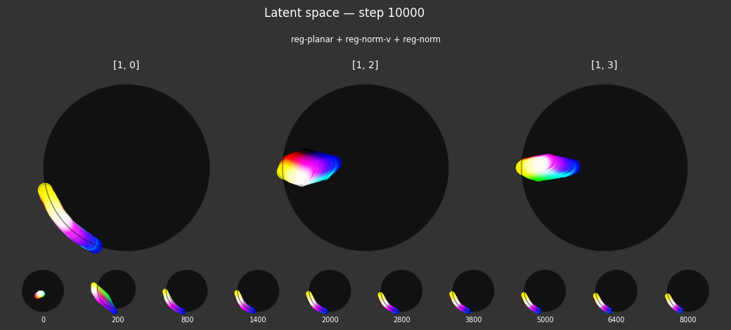
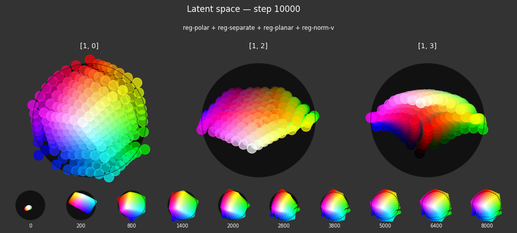
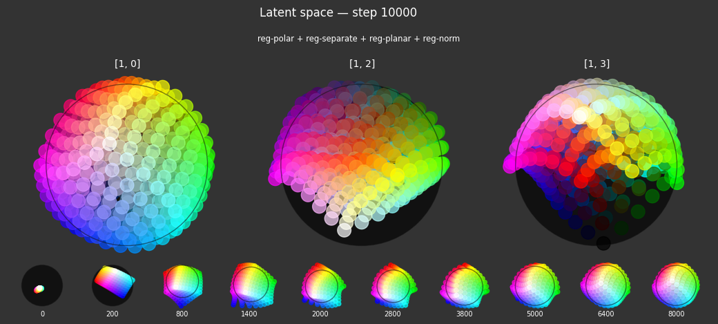
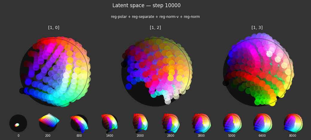
Observations

Each regularizer appears to do what we expected.

• Without reg-separate, the points all bunch up on one side of the sphere (due to reg-norm)
• Without reg-norm, the points are bunched up in the middle of the sphere
• Without reg-planar, the hues are represented in dimensions other than the first two
• Without reg-anchor, red isn't situated at $1,0,0,0$

It's unclear whether both reg-norm and reg-norm-v are needed (they both apply the unitarity constraint, but -v only applies it to the saturated hues). One interesting thing is that when only one of them is used, the resulting structure still has radius $~1$ but is more cube-like. Our understanding is that in nGPT, downstream transformer layers need unit-length vectors to do good Q-K lookups (so not required in this simple MLP architecture).

In nGPT, the activations are explicitly normalized to have unit length, instead of using a unitarity regularization term. We chose to use regularization because we feel that normalization probably hides too much of the goal from upstream layers. Consider: if you only normalize, then the "true" representations might be bunched in the middle of the hypersphere, arbitrarily close to the origin. If a point was too close to the origin, small perturbations could cause it to flip to another side of the sphere. So we expect that the model will perform better on its primary objective if the upstream representations are as close as possible to what the downstream layers expect.

The network probably needs extra capacity to form the sphere. A good trade-off might be to use very a weak unitarity term, so that it is regularized toward a radius one hypercube, and then explicitly normalized to a unit hypersphere.