Drafted 2026-09-23; adopted 2026-09-25 after five review rounds. A change to which concept D2.2 anchors. The machinery stays the same, and so do the claims in the design, whose quick route puts the experiments below in order.
In short: ex-2.2.14 anchored an op, but the anchor went to the word that names the op. We propose taking op words out of the grammar, so that the model has to work out the op from a few solved examples. That is closer to what M3, the next milestone, needs: it applies SCA to language models, where the concepts we care about are inferred from context and have no word of their own.
Ex-2.2.14 anchored difference and every gate passed. The anchor concentrated on the op word embedding: the pull put it on e₁ at a cosine near 1, and the op position stays there at every slice. When only the op word was pulled, the blocks passed a twentieth of that alignment on to = and none of it to the answer.
So the anchored concept was an attribute of one token: which op this word names. That is the D2.1 result again, with a categorical attribute in place of a graded one. Suppression at the op word will very likely remove the op, but deleting the word token would do the same, so it cannot show what anchoring adds. The dose axis of the projection also collapses there: its re-normalizing gain, 1/√(1−x₁²), is unbounded at full alignment, so a state that is all concept has no partial dose.
Every op in the current grammar is named by a word, so choosing a different op will not change this.
The lead target for M3 is sycophancy. No single token names it. It is inferred from the context and used far from where its evidence appears, and its labels will be scarce and noisy. Before M3, D2.2 should tell us:
The current design answers (4), with the caveat that a scarce labeller only had to find one embedding row. It answers (2) only in the token-mask sense, and leaves (1) unmeasured.
The concept here is the task the model is asked to do, while sycophancy is a behavior conditioned on cues observed earlier in a conversation, which stay in force until something changes them. The topic markers sketch would be a step toward that, and it is deferred.
And everything here trains from scratch. A pretrained model already has a task direction of its own (see the function-vector work below), so anchoring at fine-tune time would have to move a concept the model has already placed. This grammar could test that too, by fine-tuning an unanchored control with the anchor term; it is listed under open questions.
We take the op word out of the grammar. Each line is one context: a few solved examples of one op, written with a neutral symbol in place of the op word, then a query under the same op:1
red ? cyan = white, c999 ? c666 = c333, yellow ? red =
Here the op is difference. The first example fits four ops and the second fits two, and difference is the only op that fits both, so the model can work it out and answer lime. Op words never appear in the corpus, so the op is always inferred; a corpus that sometimes named it would give the anchor a token to attach to again.
The symbol ? stays constant, and stands for "some op". It has no information of its own, so the frame would work without it, but it keeps the shape of each equation close to the current grammar. It also gives the model a position between the operands that it may use for its own computation, perhaps to gather the op; whether it does is an open question.
The op becomes a latent task that the model infers from examples. The anchored concept is "the op in this context is difference", and no token names it.
One context per line keeps the line as the unit the existing code counts in: the holdouts and per-line scoring count contexts, and the labeller can draw once per context. That needs a new keying. op keying draws once per line, but reads the op off the op word, which is gone, and line keying draws on the colors. The new keying reads the op of each context from an array stored beside the corpus, one entry per line. It also keeps the eval to one line per forward pass, so the packed-context leakage item stays an M3 question. Training windows still see the previous lines, which hold other contexts with independent ops. The model would likely learn to ignore them, and an attention mask that resets at \n would make that certain.
Lines get longer, from 6 tokens to about 20 with three examples, and their length can vary. The code finds the line and role of a token by arithmetic on a fixed length (LINE_TOKENS, 6 today: line = position ÷ 6, role = position mod 6). A variable length needs two integer arrays the size of the corpus instead, the line and role of every token, computed once from the positions of \n. That needs a little memory and no padding. Training windows are random crops of the packed corpus, so the first context in a window is usually cut short; the block size should fit at least two whole contexts. At 64 tokens today, that is about two contexts and a fragment, so the block size will likely need to grow.
For any context, the posterior over ops given the examples can be computed from the op table: how likely each op is to have produced the answers shown. That gives us three things to design with:
difference, which plays the part redness played for red;difference: the answer distribution weighted by the posterior, with difference removed and the rest renormalized;The posterior uses the same rounding as the corpus. The corpus rounds stochastically, so the answer to an example is a draw from up to eight colors, and the likelihood of a shown answer under an op is the probability that the rounding of that op gives it (answer_dist in sca.data.ops).2 Under replacement op noise (below) the likelihood also includes the noise: with rate ρ, it is 1 − ρ times the probability under the op, plus ρ times the mean probability under the other ops. This is the posterior a model trained on the noisy corpus can reach at best. It also keeps every op above zero, so the target null is defined on a context that fits difference alone: there it weights the other ops by how nearly they fit.
Clean examples would pin the op down fast. On table A+, one clean example puts a posterior above 0.95 on the true op for about half of contexts, and three examples do so for nine in ten. So the example count alone would grade very little. What does grade it is replacement op noise: showing, in some examples, the answer another op would give. With a replacement rate near 0.3 and three or four examples, the posterior on the true op spreads across the whole range. With three examples at a rate of 0.35, about a fifth of contexts are above 0.95, 45% are between 0.5 and 0.95, and 35% are below 0.5.3
Adding wrong answers drawn at random from the color cube would grade much less, because usually no op produces them: each one removes the evidence of its example without pointing anywhere else. They could still appear at a low rate, so that the model learns to discount examples that fit nothing. In every case the query (the final equation) is clean and its target is the answer under the true op, so the noisy examples are evidence to weigh, and how much the model relies on them is what the stimulus measures.
Function vectors (Todd et al., 2023, arXiv:2310.15213) and task vectors (Hendel et al., 2023, arXiv:2310.15916) study pretrained language models given in-context examples of word-to-word functions over natural concepts: antonyms, country to capital, English to French. They find the task compressed into a direction in the residual stream, moved by a few attention heads to the final position, from about the middle layers on. Those methods search for that direction after training; the SCA version would place it during training. We keep the color domain: their tasks need the knowledge of a pretrained model, and ours keeps a computable posterior, the op table, and the checkpoints and machinery we already have.
Their results suggest mid-depth, at the position where the answer forms, which for us is the query =. That is a place to look first, and a weak prior on where the op lives: it may be assembled earlier, at the query ? or across the examples, or stay spread out. So the label is a binary one on the whole context, which is likely also the form an M3 labeller can give, and where the anchor ends up is something we measure.
difference on the stored ex-2.2.14 checkpoints. Scoring only, as planned in the design: the op-word edit against a token mask, and the use-site edits on the whole-line primary. It turns "the anchor is a token" into a measurement. Its outcome decides how much of the old line to report, and it does not decide whether to pivot: if the use-site edits move the answer, that is a result worth writing up beside the pivot, and only the new grammar can show whether SCA anchors a concept the model computes.The quick route in the design trains step 2 and the first reads of step 3 in one pilot, and runs step 1 while the grammar is built.
With the op inferred, no model can do better than answering with the answer distribution weighted by the posterior. That limit, the Bayes ceiling, can be computed for every context, and it is well below 1. With three clean examples we expect about three in four answers to be right, and almost all of the shortfall comes from stochastic rounding: a model told the op would score about the same. Replacement op noise adds a shortfall that comes from inference. At three examples and a rate of 0.35, the ceiling falls to about 0.6, while a model told the op would still score about 0.75.3 So the task gate would be the distance of the control from the ceiling, in place of the old accuracy numbers, and the report would show the ceiling for a model told the op beside it, so that the part of the gap due to inference can be seen.
A calibration check is needed: does the answer distribution of the model match the one weighted by the posterior? That would show whether the model weighs every example appropriately.
That check may cause us to change the plan. For each example the model has to know what all eleven ops would give for that pair, keep the ops that fit, and pool over examples. That is more work than applying a named op. We expect d64-L4 to be enough, since there are no variables to track, but that is untested. If the control cannot get near the ceiling, the next step would be a wider or deeper control before anything is anchored.
Verification (D2.3) could be trained here from the start or added later as a fine-tuning stage; discussed below.
= and the answer), or only past the embedding slice. This is cheap in compute, but the model can copy the op word to = through attention, which makes it a lookup one hop later, and finding that out would take a round. Dropped.The model might key on a surface feature that correlates with the op, such as a characteristic answer color. #215 found a case of this kind on the old grammar, where the untied readout made e₁ a "syntax word comes next" feature. The posterior makes this checkable: a context whose examples fit two ops equally well should give an intermediate alignment, and a shortcut would likely not follow it.
This may happen along two axes:
Still, we will need to tolerate incorrect labels too, since M3 labels will be noisy. A strong pull on those states could hurt the task or teach a shortcut. The pooled anchor term4 should soften the position axis, but it does nothing for the evidence axis.
The binary whole-line label stays the default, since it is likely the form an M3 labeller can give. Four cheap label variants should measure the effect:
(a) leave out the embedding slice;
(b) pull only the latter half of each line, where the posterior given the prefix is at or near its final value;
(c) label a position when the posterior given the tokens before it clears a threshold, which handles both axes and is the form an M3 labeller with a confidence cutoff would give;
(d) label each context with probability equal to its posterior on difference, so the labels follow the evidence the model can see.
The model never sees a label, so none of these gives it a way to read the answer from the label. Variant (d) would pull each context, on average, in proportion to its posterior, which trains the grading that the graded stimulus is meant to show; so alignment in the middle band would no longer be a result that the pull left free.
? saturatesThe pooled pull concentrates where alignment comes most easily, and the query ? is a constant token with nothing else to hold, so the model may push it to a cosine near 1 on e₁ for labelled contexts. That would still be an inferred op, computed from the examples through attention, but it would bring back the dose collapse ex-2.2.14 found at the op word, at that one position. Suppressing at ? and at the use sites separately would show whether the answer depends on that position (the bypass test from the design).
If it happens, the anchor term has options:
(a) cap the pull with a hinge that is zero above a target alignment, so no state is asked to be all concept;
(b) a larger τ, which spreads the pull over the line;
(c) a mask that pulls only positions that also hold something else, such as = and the answer.
The eval contract and the intervention library (sca.intervention: projection, reflection, repulsion, weight ablation); the fallback term, which worked on red in ex-2.2.2 and whose null now comes from the posterior; the labellers, with a new keying that labels one context, all of its examples and the query; the untied readout; the op table A+ and its op-relevance, which now decide how many examples it takes to pin down an op; and the scoring conventions from ex-2.2.9 onward. The red line of work is finished as a D2.2 prerequisite and needs nothing more for this.
D2.3 asks whether suppression can degrade completion while verification survives: the analogue of a model that can recognize a behavior without producing it. With this pivot, the concept for D2.3 would become the latent op. Completion means answering the query under the inferred op, and verification means judging whether a candidate equation follows it.
That is closer to M3 than red is, since both tasks depend on a concept the model infers from context. The shape is still quite different: here the model judges one equation against a pattern set by a few examples, while in M3 it would judge whether a whole response is, for example, sycophantic.
A verification line has the same examples, then a candidate equation with its answer, then a verdict. These are two lines, each wrapped here to fit:
red ? cyan = white, c999 ? c666 = c333,
yellow ? red = lime | TRUE

red ? cyan = white, c999 ? c666 = c333,
yellow ? red = yellow | FALSE
A FALSE candidate shows the answer another op would give, or a color from the cube, which are the two noise families the examples already have. So verification is the discounting the model already does on noisy examples, made explicit at one position.
The candidate answer of a FALSE line is wrong on purpose, so the language-model loss would be masked there.5 Otherwise verification lines would train the completion circuit toward wrong answers at the = that the completion claims read, and the model cannot tell the two kinds of line apart until the marker.
The marker | tells the model that the equation before it was the candidate and that a verdict comes next. Without it, the position after the candidate answer could be followed by another example, a verdict, or a newline, and the model could not tell which. With the marker only before the verdict, everything up to the candidate answer looks like an ordinary context with a noisy example, so the model cannot tell a verification line from a completion line until the marker arrives. A marker at the start of the line would tell the model sooner, and could change what it computes at every position; whether that matters is an open question.
We can think of three ways a model could verify. The names are ours, coined for this doc rather than terms of art, and there may be others; a model could also combine them.
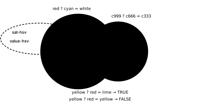
= as completion does, then compare it with the shown answer. Under causal attention this is likely the default, since the completion circuit runs at every =. It shares everything with completion, so suppressing the op likely breaks both.TRUE when one of those also fits the candidate. This route never has to settle on one op, so it might survive an anchor that holds the chosen op at the query.FALSE when no op produces the candidate at all. This needs nothing from the context, so it catches the random-cube candidates and misses the ones another op would give. So most FALSE candidates should show the answer of another op, or this route alone would score well and tell us nothing about the op.The figure shows route 2 on the two lines above.
The two examples overlap only on difference. The ops that fit lime reach that overlap, so that candidate is TRUE. The ops that fit yellow touch the first example only, so it is FALSE; with the first example alone, it would have passed.
Suppressing at the query sites and checking whether verification falls with completion should tell routes 1 and 2 apart. Seeds may split between the routes, so the effect of the intervention on verification could vary across seeds. Which route a model learns depends on a loss landscape we cannot see in advance, so the prereg should allow for either route and for a split, without predicting one. Under a whole-line label the pull also reaches the example positions, which would anchor both routes.
Verification is our measure of recognition, which is the ability M3 would want to keep. Under route 1 it would be production by another name, so the route decides whether verification measures recognition at all. A much larger model could have more routes than ours, so the route our model takes is a result about this model rather than a prediction about language models.
The asymmetry question gets harder, and more informative. Both tasks have to infer the same op from the same context. If they use one shared state, suppression would hit both, and the asymmetry would have to come from confining the anchor to the part of the stream only completion uses: the query positions and the later slices, where the op is perhaps selected and applied. We hope confining by depth alone is enough, without restricting the anchor to the query positions too. That is the open confinement item, which moves from optional to central. With the op word in the grammar, the question would have been easier to answer and would have told us little.
The later slices make depth the second axis for the split. Pretrained language models show a block structure in depth: the similarity between the hidden states of each pair of layers, measured with CKA,6 falls into an early block and a late block, with a sharp change about halfway through (Lad, Gurnee & Tegmark, 2024, arXiv:2406.19384). The authors read the early block as building features and the late block as turning them into a prediction of the next token. If verification can run on the early features and completion needs the late prediction, depth is where an asymmetry could come from. Under route 1, a depth split is unlikely to help on its own: the comparison needs the predicted answer, which the late slices produce, and the verdict is production too. It could help under route 2, where the comparison runs on sets of ops that fit, which are likely early features. So depth and route are one question.
The layer sweep would answer it for completion first: the slice at which suppression stops having an effect may be where the answer forms. The same similarity between slices is cheap to compute on our checkpoints, in the style of the geometry reanalysis, and would show whether a four-block model has such blocks at all. We would not expect it to, in a model this shallow.
Verification could be trained with completion from the start, or added later as a fine-tuning stage.
From the start, D2.3 may reuse the D2.2 checkpoints, and a no-verification arm on the control and the anchored primary would show what the extra task changes in the representations.
As a second stage, the D2.2 model stays simpler, and the anchor has to hold while a new task is learned on top of it, which is closer to how M3 would work. It would also be a version of the fine-tune test raised above. But a model fine-tuned onto a working completion circuit would likely take route 1, which reuses that circuit, and route 1 is the one where the asymmetry is least likely to appear.
The concept swap gets a natural form. Redirecting one inferred op to another is "make the model act as if the examples showed op Y". It is the steering claim M3 would want (steer from sycophantic toward candid), and the posterior still gives per-context ground truth.
? for computation. A control trained without it would say whether the frame needs it, and the states at the query ? are a candidate site for the op.This is a possible variation on the grammar, and not part of the plan. A marker sets the op for the examples that follow it, until another marker replaces it, and each marker stands for an op that is inferred as before. This is one line, wrapped here to fit:
a: red ? blue = magenta, b: red ? blue = purple,
a: white ? cyan = red, yellow ? red =
Here a is difference and b is mix. The query has no marker of its own, so it takes the op of the most recent one, much as a topic marked with the Japanese は stays in force, unrepeated, until a new one replaces it. That is closer to M3, where the relevant behavior depends on cues earlier in a conversation that stay in force until something changes them. It is also a binding task, the kind of state tracking the current grammar does not ask for, so it may need a larger model.
The corpus spells every color as a grid code (cf00 for red). This doc uses a name where the color has a familiar one, and the code otherwise: the grays here are c999, c666, and c333. ↩
A posterior computed with nearest rounding would be sharper than the corpus supports. ↩
From a scratch simulation. A scouting report would put these, and the task ceiling below, into figures. ↩↩
The pooled term asks each labelled line to align somewhere in its span, through a soft maximum over positions with temperature τ. So the pull concentrates where alignment comes most easily, and early positions are not pulled hard, except in a line whose end a training window cuts off. ↩
This matches supervised fine-tuning of language models, where the text being judged is in the prompt and has no loss. Pretraining masks nothing, but a wrong answer in a document is often flagged before it appears, which is closer to a marker at the start of the line. ↩
Centered kernel alignment: a similarity score between two sets of representations of the same inputs. Rotating either set leaves it unchanged, so it can compare layers whose coordinates mean different things. ↩