Experiment 2.7: Delete hue subspace
In Ex 2.6, we demonstrated that we could delete a single axis: warmth (red-cyan). That happened to be possible because we had regularized the model such that warmth was axis-aligned¹. We anticipate that in practice, some concepts may not fit neatly into one axis: indeed our model represents hue in two dimensions (one of which is warmth). So in this experiment, we will see whether we can ablate a multi-dimensional concept.
Hypothesis
Our model has learnt to represent hue in the first two dimensions of latent space. If we ablate the weights related to those activation dimensions, then the model should lose the ability to operate on hue. The result should be high loss across all vibrant colors, and low loss on unsaturated colors.
¹ Although warmth is isolated to a single dimension, I'm not sure if it's right to say that it's monosemantic: it's part of a linear space that happens to be axis-aligned.
from __future__ import annotations

nbid = '2.7'  # ID for tagging assets
nbname = 'Ablate hue'
experiment_name = f'Ex {nbid}: {nbname}'
project = 'ex-preppy'
# Basic setup: Logging, Experiment (Modal)
import logging

import modal

from infra.requirements import freeze, project_packages
from mini.experiment import Experiment
from utils.logging import SimpleLoggingConfig

logging_config = (
    SimpleLoggingConfig()
    .info('notebook', 'utils', 'mini', 'ex_color')
    .error('matplotlib.axes')  # Silence warnings about set_aspect
)
logging_config.apply()

# This is the logger for this notebook
log = logging.getLogger(f'notebook.{nbid}')

run = Experiment(experiment_name, project=project)
run.image = modal.Image.debian_slim().pip_install(*freeze(all=True)).add_local_python_source(*project_packages())
run.before_each(logging_config.apply)
None  # prevent auto-display of this cell
Regularizers
Like Ex 2.6:
- Anchor: pins
redto $(1,0,0,0)$ - Separate: angular repulsion to reduce global clumping (applied within each batch)
- Planarity: pulls vibrant hues to the $[0, 1]$ plane
- Unitarity: pulls all embeddings to the surface of the unit hypersphere, i.e. it makes the embedding vectors have unit length.
No change.
import torch

from mini.temporal.dopesheet import Dopesheet
from ex_color.loss import Anchor, Separate, Unitarity, RegularizerConfig, Planarity

from ex_color.training import TrainingModule

RED = (1, 0, 0, 0)

ALL_REGULARIZERS = [
    RegularizerConfig(
        name='reg-unit',
        compute_loss_term=Unitarity(),
        label_affinities=None,
        layer_affinities=['encoder'],
    ),
    RegularizerConfig(
        name='reg-anchor',
        compute_loss_term=Anchor(torch.tensor(RED, dtype=torch.float32)),
        label_affinities={'red': 1.0},
        layer_affinities=['bottleneck'],
    ),
    RegularizerConfig(
        name='reg-separate',
        compute_loss_term=Separate(power=100.0, shift=True),
        label_affinities=None,
        layer_affinities=['bottleneck'],
    ),
    RegularizerConfig(
        name='reg-planar',
        compute_loss_term=Planarity(),
        label_affinities={'vibrant': 1.0},
        layer_affinities=['bottleneck'],
    ),
]
from functools import partial
from torch import Tensor
from torch.utils.data import DataLoader, TensorDataset, WeightedRandomSampler
import numpy as np

from ex_color.data.color_cube import ColorCube
from ex_color.data.cube_sampler import vibrancy
from ex_color.data.cyclic import arange_cyclic
from ex_color.labelling import collate_with_generated_labels


def prep_data() -> tuple[DataLoader, Tensor]:
    """
    Prepare data for training.

    Returns: (train, val)
    """
    hsv_cube = ColorCube.from_hsv(
        h=arange_cyclic(step_size=10 / 360),
        s=np.linspace(0, 1, 10),
        v=np.linspace(0, 1, 10),
    )
    hsv_tensor = torch.tensor(hsv_cube.rgb_grid.reshape(-1, 3), dtype=torch.float32)
    vibrancy_tensor = torch.tensor(vibrancy(hsv_cube).flatten(), dtype=torch.float32)
    hsv_dataset = TensorDataset(hsv_tensor, vibrancy_tensor)

    labeller = partial(
        collate_with_generated_labels,
        soft=False,  # Use binary labels (stochastic) to simulate the labelling of internet text
        red=0.5,
        vibrant=0.5,
    )
    # Desaturated and dark colors are over-represented in the cube, so we use a weighted sampler to balance them out
    hsv_loader = DataLoader(
        hsv_dataset,
        batch_size=64,
        num_workers=2,
        sampler=WeightedRandomSampler(
            weights=hsv_cube.bias.flatten().tolist(),
            num_samples=len(hsv_dataset),
            replacement=True,
        ),
        collate_fn=labeller,
    )

    rgb_cube = ColorCube.from_rgb(
        r=np.linspace(0, 1, 8),
        g=np.linspace(0, 1, 8),
        b=np.linspace(0, 1, 8),
    )
    rgb_tensor = torch.tensor(rgb_cube.rgb_grid.reshape(-1, 3), dtype=torch.float32)
    return hsv_loader, rgb_tensor
import wandb
from ex_color.model import CNColorMLP


# @run.thither(env={'WANDB_API_KEY': wandb.Api().api_key})
async def train(
    dopesheet: Dopesheet,
    regularizers: list[RegularizerConfig],
) -> CNColorMLP:
    """Train the model with the given dopesheet and variant."""
    import lightning as L
    from lightning.pytorch.loggers import WandbLogger

    from ex_color.seed import set_deterministic_mode

    from utils.progress.lightning import LightningProgress

    log.info(f'Training with: {[r.name for r in regularizers]}')

    seed = 0
    set_deterministic_mode(seed)

    hsv_loader, _ = prep_data()

    model = CNColorMLP(4)
    total_params = sum(p.numel() for p in model.parameters() if p.requires_grad)
    log.debug(f'Model initialized with {total_params:,} trainable parameters.')

    training_module = TrainingModule(model, dopesheet, torch.nn.MSELoss(), regularizers)

    logger = WandbLogger(experiment_name, project=project)

    trainer = L.Trainer(
        max_steps=len(dopesheet),
        callbacks=[
            LightningProgress(),
        ],
        enable_checkpointing=False,
        enable_model_summary=False,
        # enable_progress_bar=True,
        logger=logger,
    )

    print(f'max_steps: {len(dopesheet)}, hsv_loader length: {len(hsv_loader)}')

    # Train the model
    try:
        trainer.fit(training_module, hsv_loader)
    finally:
        wandb.finish()
    # This is only a small model, so it's OK to return it rather than storing and loading a checkpoint remotely
    return model


async with run():
    model = await train(Dopesheet.from_csv(f'./ex-{nbid}-dopesheet.csv'), ALL_REGULARIZERS)
I 6.9 no.2.7: Training with: ['reg-unit', 'reg-anchor', 'reg-separate', 'reg-planar']
INFO: Seed set to 0
I 6.9 li.fa.ut.se:Seed set to 0
I 6.9 ex.se:   PyTorch set to deterministic mode
INFO: GPU available: False, used: False
I 6.9 li.py.ut.ra:GPU available: False, used: False
INFO: TPU available: False, using: 0 TPU cores
I 6.9 li.py.ut.ra:TPU available: False, using: 0 TPU cores
INFO: HPU available: False, using: 0 HPUs
I 6.9 li.py.ut.ra:HPU available: False, using: 0 HPUs
max_steps: 3001, hsv_loader length: 57
wandb: Currently logged in as: z0r to https://api.wandb.ai. Use `wandb login --relogin` to force relogin
./wandb/run-20250906_020231-gpu2wx8y
Starting phase: Train
INFO: `Trainer.fit` stopped: `max_steps=3001` reached.
I 24.2 li.py.ut.ra:`Trainer.fit` stopped: `max_steps=3001` reached.
Run history:
| epoch | ▁▁▁▂▂▂▂▂▂▃▃▃▃▃▄▄▄▄▅▅▅▅▅▅▅▆▆▆▆▆▆▇▇▇▇▇▇▇██ |
| train_loss | █▄▄▆▆▃▃▂▄▃▂▆▄▃▄▄▂▃▃▃▂▂▂▃▃▂▂▁▁▁▁▁▁▁▁▁▁▁▁▁ |
| train_recon | █▂▂▂▂▁▁▁▂▂▂▂▂▂▂▂▂▂▂▂▁▂▂▂▁▁▁▁▁▁▁▁▁▁▁▁▁▁▁▁ |
| train_reg-anchor | ▁▁▁█▁▂▁▁▁▁▁▁▂▁▁▁▁▁▁▁▁▁▁▁▁▁▁▁▂▂▁▁▁▂▁▁▂▁▁▁ |
| train_reg-planar | ▁▅▁▂█▃▁▁▁▁▁▁▂▁▂▁▁▁▁▁▂▁▁▁▂▁▁▁▁▁▁▁▁▁▁▁▁▁▁▂ |
| train_reg-separate | █▆█▆█▆▆▄▅▃▃▄▅▁▆▂▄▂▅▂▃▁▄▄▃▂▁▂▃▃▂▄▃▂▂▃▂▃▄▄ |
| train_reg-unit | █▇▆▃▂▁▂▁▁▁▁▁▁▁▁▁▁▁▁▁▁▁▁▁▁▁▁▁▁▁▁▁▁▁▁▁▁▁▁▁ |
| trainer/global_step | ▁▁▁▂▂▂▂▂▃▃▃▃▃▃▄▄▄▄▄▄▅▅▅▅▅▆▆▆▆▆▆▇▇▇▇▇████ |
Run summary:
| epoch | 52 |
| train_loss | 3e-05 |
| train_recon | 3e-05 |
| train_reg-anchor | 0 |
| train_reg-planar | 0.05332 |
| train_reg-separate | 0.43601 |
| train_reg-unit | 0.00924 |
| trainer/global_step | 2999 |
View project at: https://wandb.ai/z0r/ex-color-transformer
Synced 5 W&B file(s), 0 media file(s), 0 artifact file(s) and 0 other file(s)
./wandb/run-20250906_020231-gpu2wx8y/logs
The charts and loss values from training look much the same as last time.
- Roughly the same shape overall
- All loss values roughly the same
from ex_color.inference import InferenceModule


async def infer(
    model: CNColorMLP,
    test_data: Tensor,
) -> Tensor:
    """Run inference with the given model."""
    import lightning as L

    inference_module = InferenceModule(model, [])
    trainer = L.Trainer(
        enable_checkpointing=False,
        enable_model_summary=False,
        enable_progress_bar=True,
    )
    reconstructed_colors_batches = trainer.predict(
        inference_module,
        DataLoader(
            TensorDataset(test_data.reshape((-1, 3))),
            batch_size=64,
            collate_fn=lambda batch: torch.stack([row[0] for row in batch], 0),
        ),
    )
    assert reconstructed_colors_batches is not None
    # Flatten the list of batches to a single list of tensors
    reconstructed_colors = [item for batch in reconstructed_colors_batches for item in batch]
    # Reshape to match input
    return torch.cat(reconstructed_colors).reshape(test_data.shape)
import torch
import numpy as np

from ex_color.inference import InferenceModule


async def infer_with_latent_capture(
    model: CNColorMLP,
    test_data: Tensor,
    layer_name: str = 'bottleneck',
) -> tuple[Tensor, Tensor]:
    module = InferenceModule(model, [], capture_layers=[layer_name])
    import lightning as L

    trainer = L.Trainer(enable_checkpointing=False, enable_model_summary=False, enable_progress_bar=False)
    batches = trainer.predict(
        module,
        DataLoader(
            TensorDataset(test_data.reshape((-1, 3))),
            batch_size=64,
            collate_fn=lambda batch: torch.stack([row[0] for row in batch], 0),
        ),
    )
    assert batches is not None
    preds = [item for batch in batches for item in batch]
    y = torch.cat(preds).reshape(test_data.shape)
    # Read captured activations as a flat [N, D] tensor
    latents = module.read_captured(layer_name)
    return y, latents
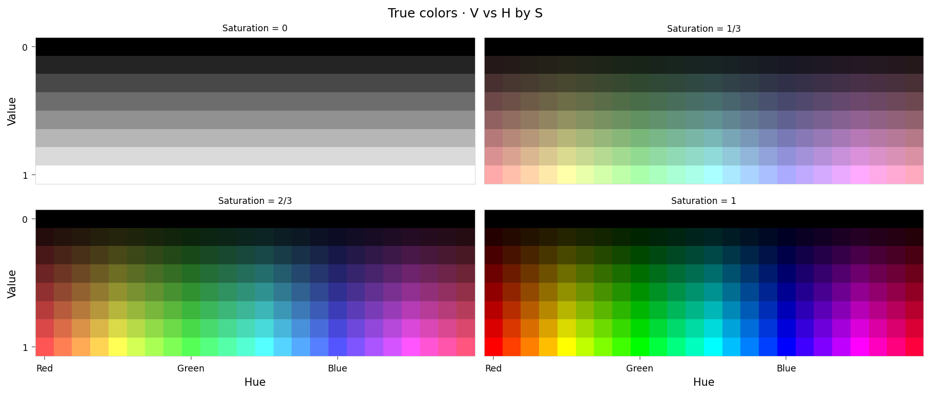
Quick sense-check: Let's see how well the trained model reconstructs colors.
from IPython.display import clear_output

import importlib
import utils.nb
import utils.plt

importlib.reload(utils.nb)
importlib.reload(utils.plt)

from ex_color.vis import plot_colors
from utils.nb import displayer_mpl


hsv_cube = ColorCube.from_hsv(
    h=arange_cyclic(step_size=1 / 24),
    s=np.linspace(0, 1, 4),
    v=np.linspace(0, 1, 8),
).permute('svh')
x_hsv = torch.tensor(hsv_cube.rgb_grid, dtype=torch.float32)

hd_hsv_cube = ColorCube.from_hsv(
    h=arange_cyclic(step_size=1 / 240),
    s=np.linspace(0, 1, 48),
    v=np.linspace(0, 1, 48),
)
hd_x_hsv = torch.tensor(hd_hsv_cube.rgb_grid, dtype=torch.float32)

rgb_cube = ColorCube.from_rgb(
    r=np.linspace(0, 1, 20),
    g=np.linspace(0, 1, 20),
    b=np.linspace(0, 1, 20),
)
x_rgb = torch.tensor(rgb_cube.rgb_grid, dtype=torch.float32)

with displayer_mpl(
    f'large-assets/ex-{nbid}-true-colors.png',
    alt_text="""Plot showing four slices of the HSV cube, titled "{title}". Each slice has constant saturation, but varies in value (brightness) from top to bottom, and in hue from left to right. The first slice shows a grayscale gradient from black to white; the last shows the fully-saturated color spectrum.""",
) as show:
    show(lambda: plot_colors(hsv_cube, title='True colors', colors=x_hsv.numpy()))
from IPython.display import clear_output
from torch.nn import functional as F

from ex_color.vis import plot_colors, plot_cube_series


interventions = []
y_hsv = await infer(model, x_hsv)
hd_y_hsv = await infer(model, hd_x_hsv)
clear_output()

with displayer_mpl(
    f'large-assets/ex-{nbid}-pred-colors-no-intervention.png',
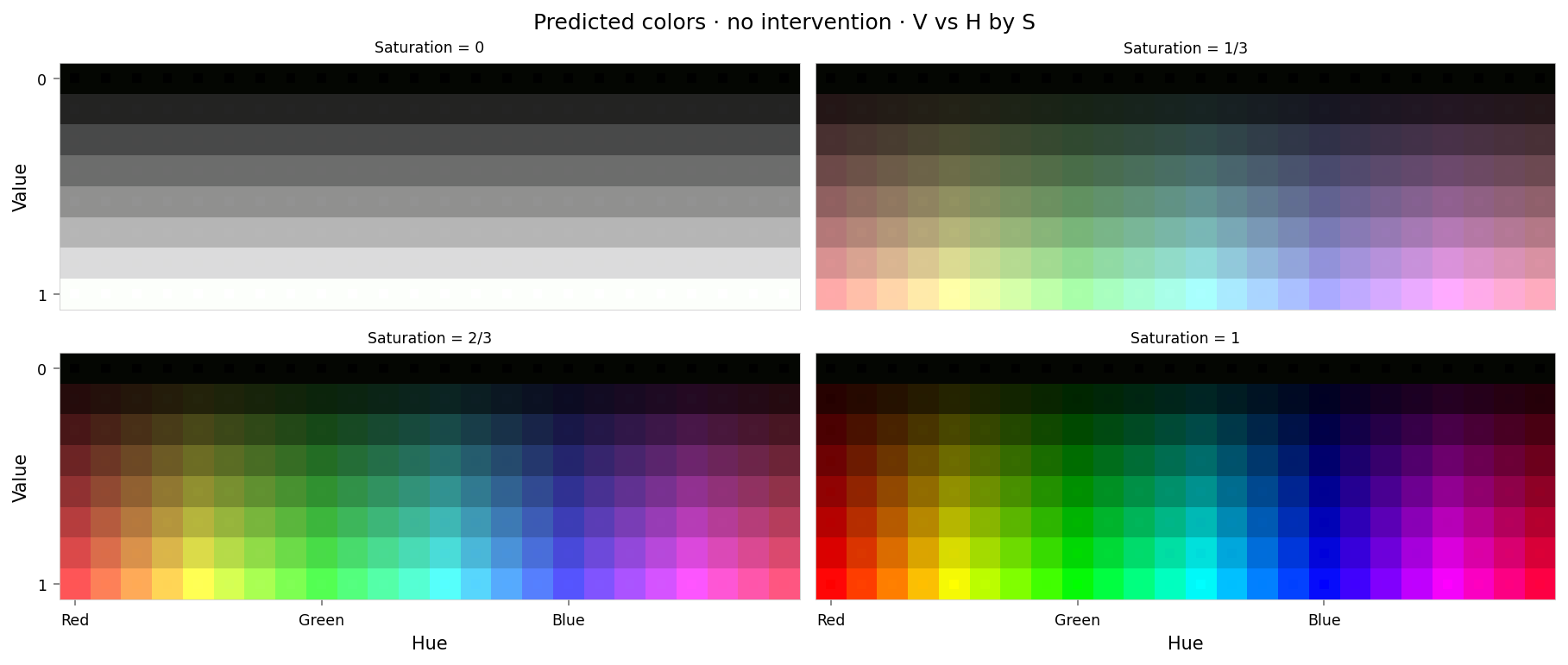
    alt_text="""Plot showing four slices of the HSV cube, titled "{title}". Nominally, each slice has constant saturation, but varies in value (brightness) from top to bottom, and in hue from left to right. Each color value is represented as a square patch of that color. The outer portion of the patches shows the color as reconstructed by the model; the inner portion shows the true (input) color. The reconstructed and true colors agree fairly well, but some slight differences are visible; for example, "white" is slightly gray, and many of the fully-saturated colors are less saturated than they should be.""",
) as show:
    show(
        lambda: plot_colors(
            hsv_cube,
            title='Predicted colors · no intervention',
            colors=y_hsv.numpy(),
            colors_compare=x_hsv.numpy(),
        )
    )

per_color_loss = F.mse_loss(hd_y_hsv, hd_x_hsv, reduction='none').mean(dim=-1)
loss_cube = hd_hsv_cube.assign('MSE', per_color_loss.numpy().reshape(hd_hsv_cube.shape))
max_loss = per_color_loss.max().item()
median_loss = per_color_loss.median().item()

with displayer_mpl(
    f'large-assets/ex-{nbid}-loss-colors-no-intervention.png',
    alt_text=f"""Line chart showing loss per color, titled "{{title}}". Y-axis: mean square error, ranging from zero to {max_loss:.2g}. X-axis: hue. The range of loss values is small, but there are two notable peaks at all primary and secondary colors (red, yellow, green, etc.).""",
) as show:
    show(
        lambda: plot_cube_series(
            loss_cube.permute('hsv')[:, -1:, :: (loss_cube.shape[2] // -5)],
            loss_cube.permute('svh')[:, -1:, :: -(loss_cube.shape[0] // -3)],
            loss_cube.permute('vsh')[:, -1:, :: -(loss_cube.shape[0] // -3)],
            title='Reconstruction error · no intervention',
            var='MSE',
            figsize=(12, 3),
        )
    )
print(f'Max loss: {max_loss:.2g}')
print(f'Median MSE: {median_loss:.2g}')

Max loss: 0.0011
Median MSE: 1.5e-05
from IPython.display import clear_output

from ex_color.vis import plot_latent_grid_3d

y_rgb, h_rgb = await infer_with_latent_capture(model, x_rgb, 'bottleneck')
clear_output()

with displayer_mpl(
    f'large-assets/ex-{nbid}-latents-no-intervention.png',
    alt_text="""Three spherical plots, titled "{title}". Each plot shows a vibrant collection of colored circles or balls scattered over the surface of a black sphere. The first plot has the appearance of a color wheel, with the full set of vibrant colors around the rim (like a rainbow), varying to black in the center. The other plots show different views of the same sphere. The last plot has hue varying across the equator and tone varying from top to bottom, and red in the center. The middle plot shows the non-hue dimensions, with brightness varying around the edge and the vibrant colors in the middle. Each ball shows the reconstructed color, with a dot in the center showing the true (input) color. In this plot the true and reconstructor colors agree fairly well, but slight differences can be seen if you look closely.""",
) as show:
    show(
        lambda theme: plot_latent_grid_3d(
            h_rgb,
            y_rgb,
            x_rgb,
            title='Latents · no intervention',
            dims=[(1, 0, 2), (2, 3, 1), (1, 3, 0)],
            dot_radius=10,
            theme=theme,
        )
    )
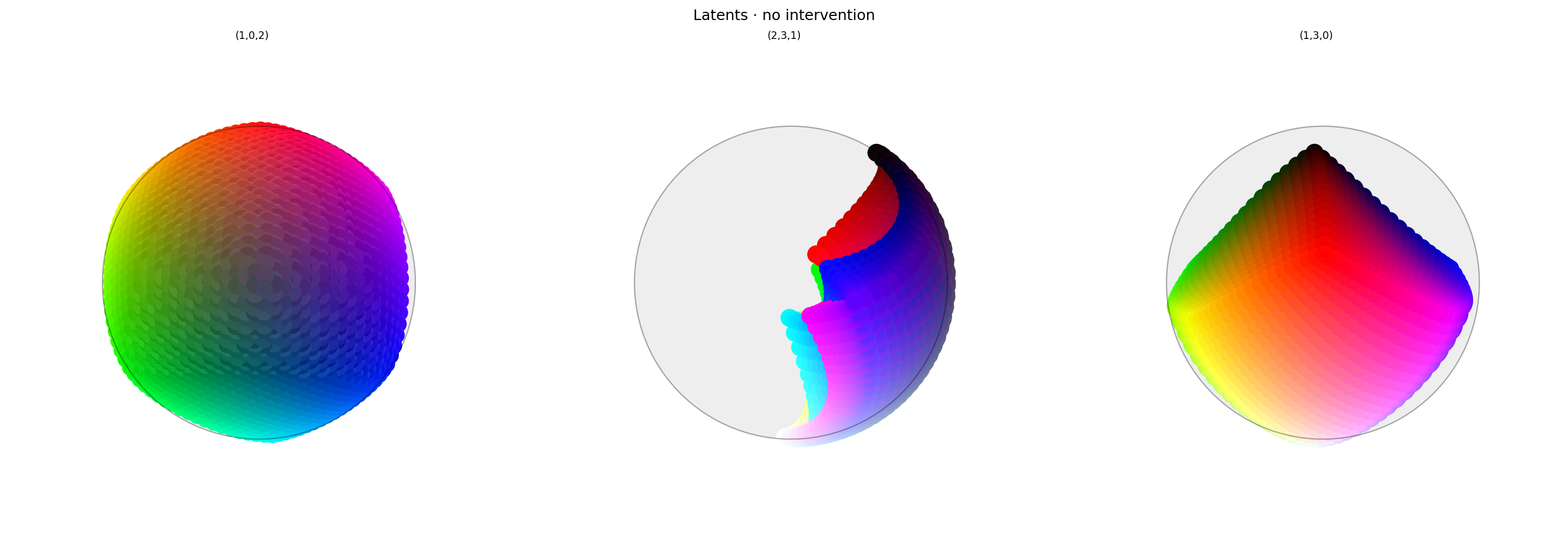
Looks fine. Note that the middle plot is rotated compared to previous experiments to show the grays along the edge of the sphere.
Ablation
Now that we have our model, let's try ablating (zeroing) hue. We'll use the same function as 2.6, but with two dimensions instead of one.
def ablate[M](model: M, layer_id: str, dims: Sequence[int]) -> M:
    """Return a copy of model where the selected latent dims are effectively nulled."""
    ...
This zeros out producer (upstream matrix) rows and consumer (downstream) columns for the given dims. Shapes remain unchanged.
from ex_color.surgery import ablate

ablated_model = ablate(model, 'bottleneck', [0, 1])

y_hsv = await infer(ablated_model, x_hsv)
hd_y_hsv = await infer(ablated_model, hd_x_hsv)
clear_output()

with displayer_mpl(
    f'large-assets/ex-{nbid}-pred-colors-ablated.png',
    alt_text="""Plot showing four slices of the HSV cube, titled "{title}". Nominally, each slice has constant saturation, but varies in value (brightness) from top to bottom, and in hue from left to right. Each color value is represented as a square patch of that color. The outer portion of the patches shows the color as reconstructed by the model; the inner portion shows the true (input) color. The reconstructed and true colors agree fairly well when the true color is desaturated or dark, but colors that should be vibrant are all grayscale.""",
) as show:
    show(
        lambda: plot_colors(
            hsv_cube,
            title='Predicted colors · ablated',
            colors=y_hsv.numpy(),
            colors_compare=x_hsv.numpy(),
        )
    )

per_color_loss = F.mse_loss(hd_y_hsv, hd_x_hsv, reduction='none').mean(dim=-1)
loss_cube = hd_hsv_cube.assign('MSE', per_color_loss.numpy().reshape(hd_hsv_cube.shape))
max_loss = per_color_loss.max().item()
median_loss = per_color_loss.median().item()
with displayer_mpl(
    f'large-assets/ex-{nbid}-loss-colors-ablated.png',
    alt_text=f"""Line chart showing loss per color, titled "{{title}}". Y-axis: mean square error, ranging from zero to {max_loss:.2g}. X-axis: hue. There are notable peak at each primary and secondary color, with slightly lower loss for ternary colors, and very low loss for black and white.""",
) as show:
    show(
        lambda: plot_cube_series(
            loss_cube.permute('hsv')[:, -1:, :: (loss_cube.shape[2] // -5)],
            loss_cube.permute('svh')[:, -1:, :: -(loss_cube.shape[0] // -6)],
            loss_cube.permute('vsh')[:, -1:, :: -(loss_cube.shape[0] // -6)],
            title='Reconstruction error · ablated',
            var='MSE',
            figsize=(12, 3),
        )
    )
print(f'Max loss: {max_loss:.2g}')
print(f'Median MSE: {median_loss:.2g}')

Max loss: 0.31
Median MSE: 0.008
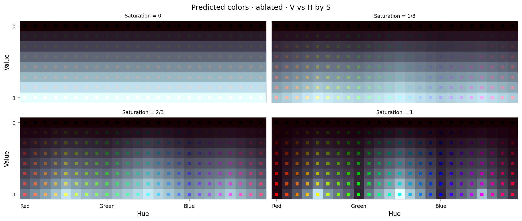
This looks like a clean ablation. The predicted colors are now entirely grayscale, even where they should be fully-saturated. The saturation and value error plots show very reasonable curves from close-to-zero (no error) at zero saturation/value, to high error at full saturation/value.
Slightly surprising:
- Error varies systematically by hue, with primary and secondary colors having higher error than ternary colors.
- Reconstructed also vary systematically: primary colors mapped to near-black, while secondary colors map to near-white, and ternary colors map to middle-gray.
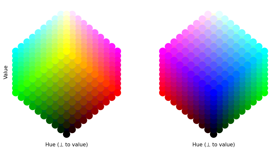
I expect this is due to the way the RGB cube maps to HSV: if you tilt the cube such that white is at the top and black is at the bottom, then:
- The primaries and secondaries are on corners around the middle, and ternaries are on the edges
- Primaries are closer to the bottom (black), and secondaries are closer to the top.
Also, numerically, primaries are full value in one channel, while secondaries are full value in two channels, i.e. primaries are composed of "more zeros" and secondaries are composed of "more ones". But I find the geometric explanation more satisfying.
from typing import cast
from matplotlib.axes import Axes
import numpy as np
import matplotlib.pyplot as plt

from ex_color.data.color_cube import ColorCube
from utils.nb import displayer_mpl


def set_alpha(colors: np.ndarray, alpha: float) -> np.ndarray:
    """Set alpha channel of colors."""
    assert colors.ndim == 2 and colors.shape[1] in (3, 4), 'colors must be [N, 3] or [N, 4]'
    if colors.shape[1] == 3:
        colors = np.concatenate([colors, np.ones((colors.shape[0], 1), dtype=colors.dtype)], axis=1)
    colors[:, 3] = alpha
    return colors


def plot_rgb_cube_orthographic(rgb_grid: np.ndarray, *, point_size: int = 30):
    """Plot RGB cube with diagonal (black→white) vertical (white on top)."""
    assert rgb_grid.ndim == 4 and rgb_grid.shape[-1] == 3, 'rgb_grid must be [R,G,B,3]'
    R, G, B, _ = rgb_grid.shape
    # Normalized coordinate for each lattice point
    r = np.linspace(0, 1, R)
    g = np.linspace(0, 1, G)
    b = np.linspace(0, 1, B)
    rr, gg, bb = np.meshgrid(r, g, b, indexing='ij')
    coords = np.stack([rr, gg, bb], axis=-1).reshape(-1, 3)
    colors = rgb_grid.reshape(-1, 3)

    # sides = ('front',)
    sides = ('front', 'back')
    fig, axs = plt.subplots(1, len(sides), figsize=(4 * len(sides), 4), sharey=True, squeeze=False)
    axs = axs.flatten()
    for i, (side, ax) in enumerate(zip(sides, axs, strict=True)):
        ax = cast(Axes, ax)

        # Build an orthonormal basis with diag as vertical axis
        diag = np.array([1.0, 1.0, 1.0])
        e3 = diag / np.linalg.norm(diag)  # vertical (black→white)
        e1 = np.array([1.0, -1.0, 0.0] if side == 'front' else [-1.0, 1.0, 0.0])
        e1 -= e1 @ e3 * e3
        e1 /= np.linalg.norm(e1)
        e2 = np.cross(e3, e1)

        projected = coords @ np.stack([e1, e2, e3], axis=1)
        x: np.ndarray
        y: np.ndarray
        z: np.ndarray  # noqa: E702
        x, y, z = projected.T  # z is vertical but we will use y= z for 2D plot

        # Sort so that lower (darker) points do not occlude brighter ones
        order = np.argsort(y)
        ax.scatter(x[order], z[order], c=colors[order], s=point_size)
        ax.set_xlabel('Hue (⊥ to value)')
        if i == 0:
            ax.set_ylabel('Value')
        ax.xaxis.set_ticks([])
        ax.yaxis.set_ticks([])
        ax.spines['top'].set_visible(False)
        ax.spines['bottom'].set_visible(False)
        ax.spines['right'].set_visible(False)
        ax.spines['left'].set_visible(False)
        ax.patch.set_alpha(1)
        ax.set_aspect('equal')

        # ax.set_title(side.capitalize())

    # fig.suptitle('RGB cube (true colors)')
    return fig


with displayer_mpl(
    f'large-assets/ex-{nbid}-rgb-cube.png',
    alt_text="""Two colorful, orthographic views of the RGB cube, rotated such that black is at the bottom and white is at the top. The other corners of the cube are arranged around the middle in two bands, one higher and one lower. The left plot, titled 'font', has in its top band cyan, yellow, and magenta, and in its bottom band green, red. The right plot, titled 'back', has in its top band magenta and cyan, and in its bottom band red, blue, and green.""",
) as show:
    show(
        lambda: plot_rgb_cube_orthographic(
            ColorCube.from_rgb(
                np.linspace(0, 1, 10),
                np.linspace(0, 1, 10),
                np.linspace(0, 1, 10),
            ).rgb_grid,
            point_size=175,
        )
    )
from IPython.display import clear_output

from ex_color.vis import plot_latent_grid_3d

y_rgb, h_rgb = await infer_with_latent_capture(ablated_model, x_rgb, 'bottleneck')
clear_output()

with displayer_mpl(
    f'large-assets/ex-{nbid}-latents-ablated.png',
    alt_text="""Three spherical plots, titled "{title}". Each plot shows a vibrant collection of colored circles or balls scattered over the surface of a sphere. The first plot has a black dot in the center, with nothing around the rim. The other plots show different views of the same sphere. The last plot has a line down the center, showing value varying from top to bottom, and is otherwise empty. The middle plot shows a similar line but around the edge of the sphere, and is empty in the middle. Each ball shows the reconstructed color, with a dot in the center showing the true (input) color. The true and reconstructed colors disagree significantly.""",
) as show:
    show(
        lambda theme: plot_latent_grid_3d(
            h_rgb,
            y_rgb,
            x_rgb,
            title='Latents · ablated',
            dims=[(1, 0, 2), (2, 3, 1), (1, 3, 2)],
            dot_radius=10,
            theme=theme,
        )
    )
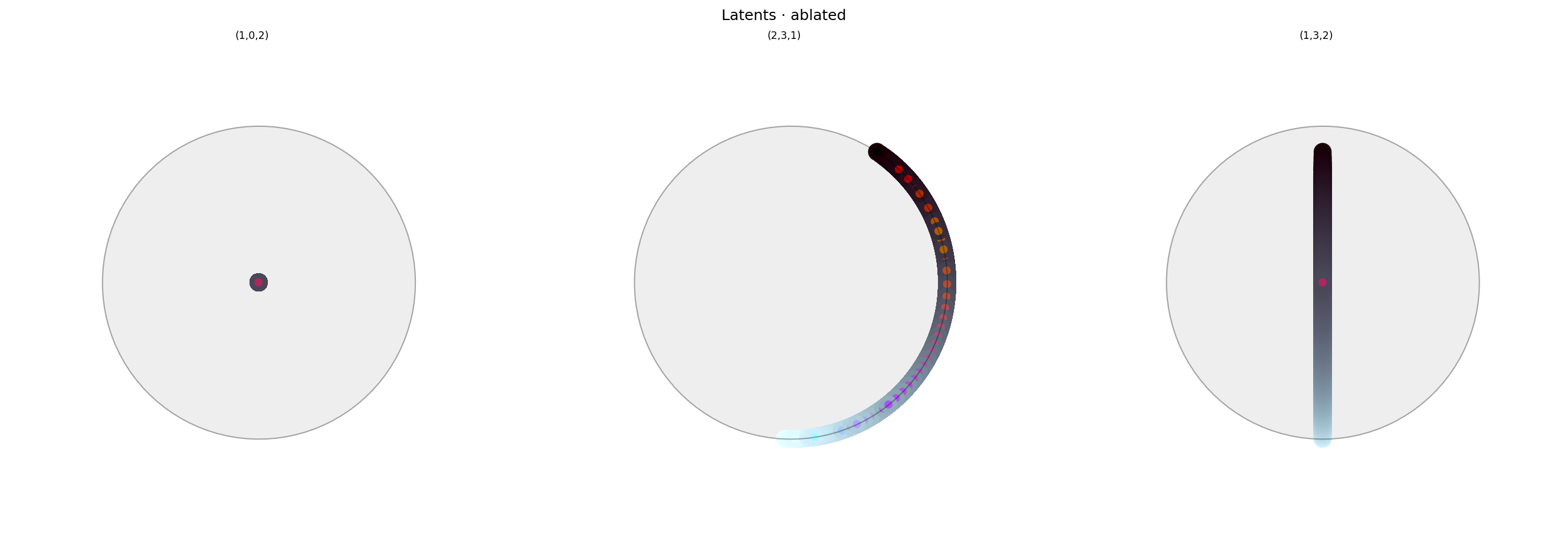
Here we clearly see that hue has been removed from latent space: only brightness is present, so the decoder should be unable to access any information about hue.